| Name | Last modified | Size | Description | |
|---|---|---|---|---|
| Parent Directory | - | |||
| plots/ | 2022-02-02 17:52 | - | ||
| programs/ | 2024-01-31 13:47 | - | ||
Each of the above is an implementation of the midpoint method. Here is the output of integration_test.m, which demonstrates the weaknesses of the first two implementations and motivates the third:
octave:1> integration_test
O = ---- 1e6 steps using midpoint0 ---- = O
err =  3.4454e-10
execution_time =  43.124
O = ---- 1e6 steps using midpoint1 ---- = O
err =  3.4454e-10
execution_time =  0.18330
O = ---- 1e8 steps using midpoint1 ---- = O
octave(95255) malloc: *** mmap(size=800002048) failed (error code=12)
*** error: can't allocate region
midpoint2.m is used in all the examples that follow. The integration is sped up by vectorizing N steps togetether, at the expense of whatever memory usage is required for an array of that size. A total of MN integration steps are taken by putting the vectorized code inside a loop with M iterations. Since interpreted loops are slow, increasing M while keeping MN constant will increase execution time but save memory.
I have done a series of test runs to characterize convergence rates and document the effects of roundoff error for several different integrands.
| M | N | test code | integrand | plot |
| 1e0-1e6 | 1e0-1e6 | integration_test1.m | improper.m | performance.pdf |
| 1e1 | 1e1-1e7 | integration_test2.m | circle.m | circleMN=1e2-1e8.pdf |
| 1e4 | 1e1-1e7 | integration_test2.m | circle.m | circleMN=1e5-1e11.pdf |
| 1e5 | 1e1-1e7 | integration_test2.m | circle.m | circleMN=1e6-1e12.pdf |
| 1e4 | 1e1-1e7 | integration_test4.m | parabola.m | parabolaMN=1e5-1e11.pdf |
| 1e1 | 1e1-1e7 | integration_test5.m | parabola.m improper.m circle.m | convergenceMN=1e2-1e8.pdf |
On my laptop, I found that N = 1e8 was too much for my memory to handle, so many of the runs were done with a range of 1e1 to 1e7 steps vectorized together.
The suite of runs with integration_test1 shows that the performance gains are minimal for N > 1000. This means that the vectorized additions are about 1000 times faster than one cycle through an interpreted for loop.
For large numbers of steps, effects of roundoff error can be seen. At best, the available accuracy bottoms out just above the machine precision. At worst, an excessive number of steps causes roundoff error to grow, diminishing accuracy.
When M is larger than N, there is more roundoff error in the for loop summation; when the opposite is true, there is more roundoff error in the vectorized summation; when N is similar in magnitude to N, the overall roundoff error of the calculation is minimized. This explains why, for example, the three different trials with integration_test2.m produced convergence plots that differ in the regions where the number of steps overlap.
Convergence rates differ significantly among the three integrands I tried (integration_test5). That's because the integrands differ in smoothness and in the magnitudes of their higher derivatives. So, when you see derivations showing some particular scaling error with the number of steps, always take it with a grain of salt!
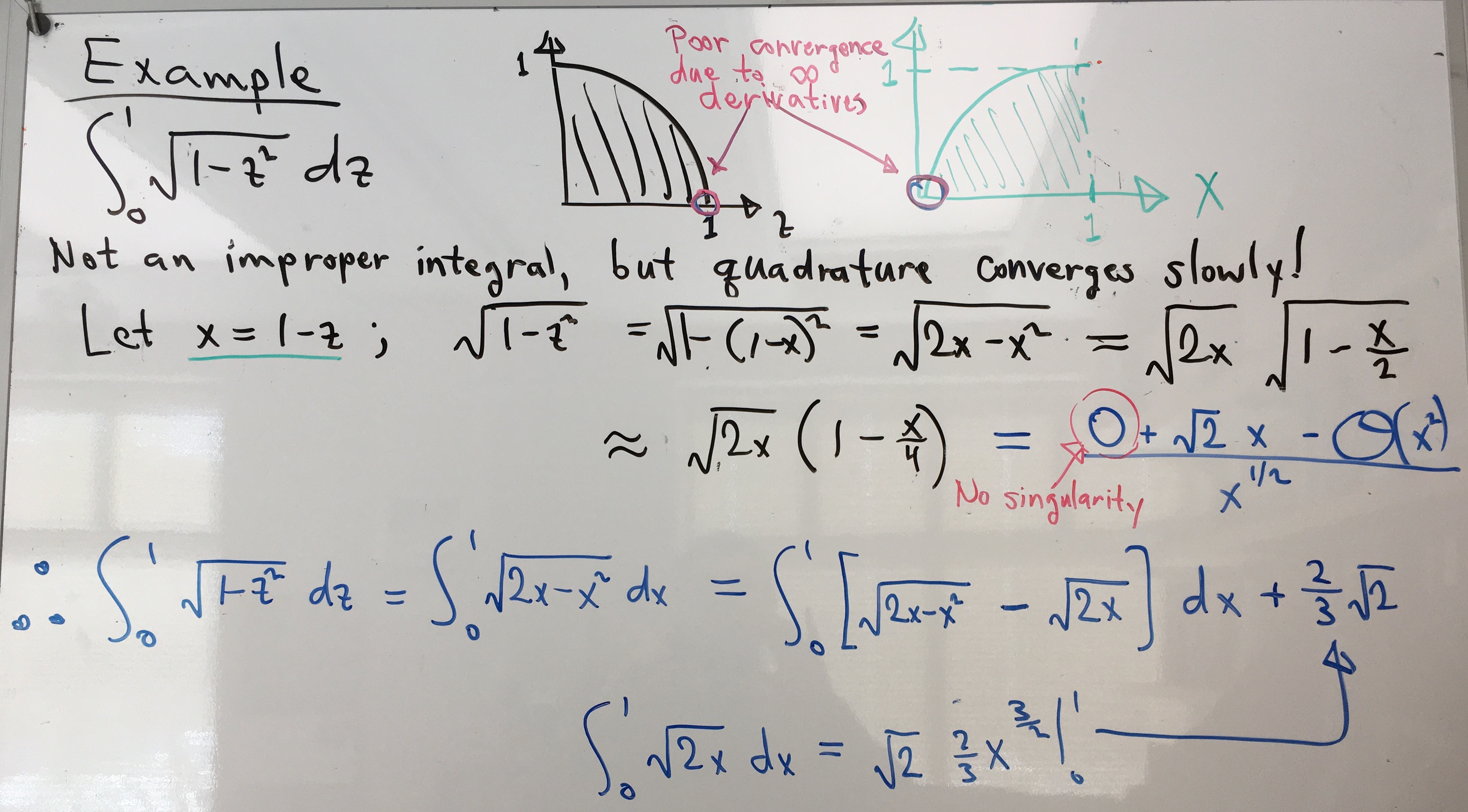
Are we stuck with slow convergence for improper integrals? No!
It is often possible to transform the integral in such a
way as to remove the singularity. There are many approaches. One example is worked out in
the notes, and we have a demo:
octave:2> integration_test6
O = ---- parabola ---- = O
Nsteps =

 Columns 1 through 6:

   1.0000e+03   1.0000e+04   1.0000e+05   1.0000e+06   1.0000e+07   1.0000e+08

 Column 7:

   1.0000e+09

Ntrials =  7
execution_time =    8.0800e-04
execution_time =    3.0000e-05
execution_time =    7.6000e-05
execution_time =    4.0200e-04
execution_time =  0.0010840
execution_time =  1.3016
execution_time =  8.9625
O = ---- improper2 ---- = O
execution_time =    1.5400e-04
execution_time =    2.2000e-05
execution_time =    2.6000e-05
execution_time =    8.9600e-04
execution_time =  0.0011080
execution_time =  3.3120
execution_time =  30.498
best_estimate =  5.2440
uncertainty =    1.4662e-04
O = ---- improper3 (transformed from improper2) ---- = O
execution_time =    1.6600e-04
execution_time =    1.7600e-04
execution_time =    1.4000e-04
execution_time =    4.2600e-04
execution_time =  0.0023240
execution_time =  4.8951
execution_time =  62.869
best_estimate =  5.2441
uncertainty =   -4.5459e-12
O = ---- Calculations complete! ---- = O
My notes go on to describe a correction that can be used when the function is not analytic (even with an integrable singularity) at one end of the interval. Let's apply this technique to our numerical integration of the quarter-circle:

The result is that we can use our simple little midpoint method to calculate pi with double precision accuracy. Demonstration:
octave:1> integration_test7
O = ---- parabola ---- = O
Nsteps =

        1000       10000      100000     1000000    10000000   100000000

Ntrials = 6
execution_time = 7.314999999999960e-03
execution_time = 5.144999999999955e-03
execution_time = 5.686000000000080e-03
execution_time = 9.036000000000044e-03
execution_time = 3.512400000000016e-02
execution_time = 0.507511000000000
O = ---- circle ---- = O
execution_time = 4.289999999999683e-03
execution_time = 4.248000000000030e-03
execution_time = 5.432000000000325e-03
execution_time = 1.298999999999984e-02
execution_time = 8.460699999999965e-02
execution_time = 1.251342000000000
estimated_error = -2.635447415855197e-12
estimate_pi = 3.141592653590140
actual___pi = 3.141592653589793
abs_error = 3.463895836830488e-13
O = ---- circle2 (transformed from circle) ---- = O
execution_time = 7.299000000000166e-03
execution_time = 5.592000000000041e-03
execution_time = 6.648000000000209e-03
execution_time = 2.294799999999997e-02
execution_time = 0.162154000000000
execution_time = 2.490312000000000
estimated_error = -4.440892098500626e-16
estimate_pi = 3.141592653589793
actual___pi = 3.141592653589793
abs_error = -4.440892098500626e-16
O = ---- Calculations complete! ---- = O
Page maintained by Charles Kankelborg