Week 1
The first week of the REU program consisted of IDL tutorials, which were given by Adam Kobelski and Roger Scott. The purpose of these was to help us get accustomed to the most important aspects of the new programming language, and become comfortable with it in preparation for the work ahead.
Week 2
Having completed the week of IDL tutorials our focus shifted towards our individual research projects. My particular project involves active region transient brightenings (ARTBs). These are similar to solar flares - insomuch as they are magnetic reconnection events - however, they have several advantageous features, which make them an attractive phenomenon to study.
Firstly, ARTBs occur at lower energies than solar flares. As a result, they also occur much more frequently, meaning that ARTBs are far more suitable for statistical analysis. Secondly, ARTBs are much smaller events, meaning that a number of complicating factors necessary when developing numerical models of solar flares can be discounted, making ARTBs easier to describe using current numerical models. Thus, ARTBs are an effective and practical way to probe magnetic reconnection kinematics without requiring overly complex models and vast amounts of computing time.
Week 4
Parse XRT Data
The data set chosen to search for ARTBs was an XRT data set from October 2011, which covered one weeks worth of observations. Since ARTBs typically evolve over far shorter time scales - a few, to tens of minutes - it was necessary to split this large data set up into smaller, more managable, chunks before searching for ARTBs.
To do this, I wrote some code to split the data into chunks between 30 mins and a few hours. In order to use the maximum amount of data, an additional criterion was imposed on the data, whereby the data would only be split when there was a suitable natural pause. Typically there are gaps in the data when the Hinode satellite cannot observe the Sun as a result of its orbital position, or when the orientation of the satellite is changed. The code keeps a running total of the elapsed time in the current image stack, then once it is greater than 30 minutes and a suitable gap appears, that image stack is saved as a new data set. The running total then resets and the process is repeated. The result is that the original week-long data set is split into 61 smaller data sets; some notes on each of these appear below.
Notes
set 01) Looks good, 90mins, 30 images [gt 15]set 02) One possilbe ARTB, blackout midway through however [gt 15]
set 03) Couple possible events, blackout in middle of one, iffy [won't run]
set 04) Good [won't run]
set 05) Good [gt 15]
set 06) Clear data, not sure if there are any events [gt 15]
set 07) Good [INVERTED]
set 08) One possibly two events, blackout part way through one though [won't run]
set 09) Good [gt 15]
set 10) Good [wont't run]
set 11) Good [gt 15]
set 12) Two bad images, maybe only one event,longer though [lt 15; only 1 ARTB]
set 13) Good images but not much activity [lt 15]
set 14) Very long, three bad images, not a lot of activity [gt 15] **
set 15) Two bad images, not a lot of activity [lt 15]
set 16) Good [INVERTED]
set 17) Good, nice bit of activity, a few darkened images but still clear [gt 15] ***
set 18) Good, nice bit of activity, couple bad images [lt 15]
set 19) Lots of activity, long, few darkened images but overall good [INVERTED]
set 20) Nice images, not a lot of activity [lt 15]
set 21) Couple of events, few bad images [no ARTBs]
set 22) Nice images, not much activity [lt 15] **
set 23) Very short, one possible event, large jump at end [cadence too low]
set 24) Nice images, long, but not much activity [gt 15]
set 25) Nice images, not much activity [no ARTBs]
set 26) One or two events, few bad images [lt 15]
set 27) Couple of events, one or two bad images [lt 15]
set 28) Good, a few nice events [lt 15]
set 29) Some decent events, long, few bad images [gt 15]
set 30) Good [lt 15]
set 31) Very little activity [lt 15]
set 32) Some activity, not great [no ARTBs]
set 33) Decent, some nice events, one or two bad images
set 34) Good, some dark images but still clear
set 35) Lots of activity, long [RUN]
set 36) Good
set 37) Good [RUN]
set 38) Good
set 39) Good
set 40) Good
set 41) Good
set 42) Good
set 43) Very short, not much use
set 44) " "
set 45) " "
set 46) " "
set 47) " "
set 48) " "
set 49) " "
set 50) " "
set 51) " "
set 52) Good
set 53) Good
set 54) Good
set 55) Good
set 56) Good
set 57) Good
set 58) Very short
set 59) Okay, looks like a solar flare, some smaller events too and a couple of bad images
set 60) Some good activity
set 61) Good
Having reviewed each of the above sets of data, the best canditates for ARTB searches were picked out - these were typically the ones with the most activity and of suitable length/cadence.
Searching for ARTBs
The program 'find_artb' was used to search the data for ARTBs. The program works by calculating the running mean of the background, then searches for pixels with a standard deviation greater than five sigma. When it finds such a pixel, it then searches all points connected to that pixel in order to determine whether they are part of the same brightening event. This effectively traces out the shape of the potential ARTB region and creates a new array containing the information about all ARTBs within the chosen image stack, and their location.
Data set 35
Output of 'find_artb' for data set 35
Upon running the ARTB search code, however, a problem was encountered: whilst processing certain data sets the code would become stuck and process individual pixels, one after another, as if they were part of an ARTB. I discussed this with Adam and he was able to modify the 'find_artb' code to fix the problem. The trouble was caused by the running mean count; it wasn't resetting properly in the longer data sets with the result that the calculated running mean was lower than should have been the case. This meant that the program was then flagging virtually all pixels as being ARTBs. A binary counting method was introduced to remedy the problem.
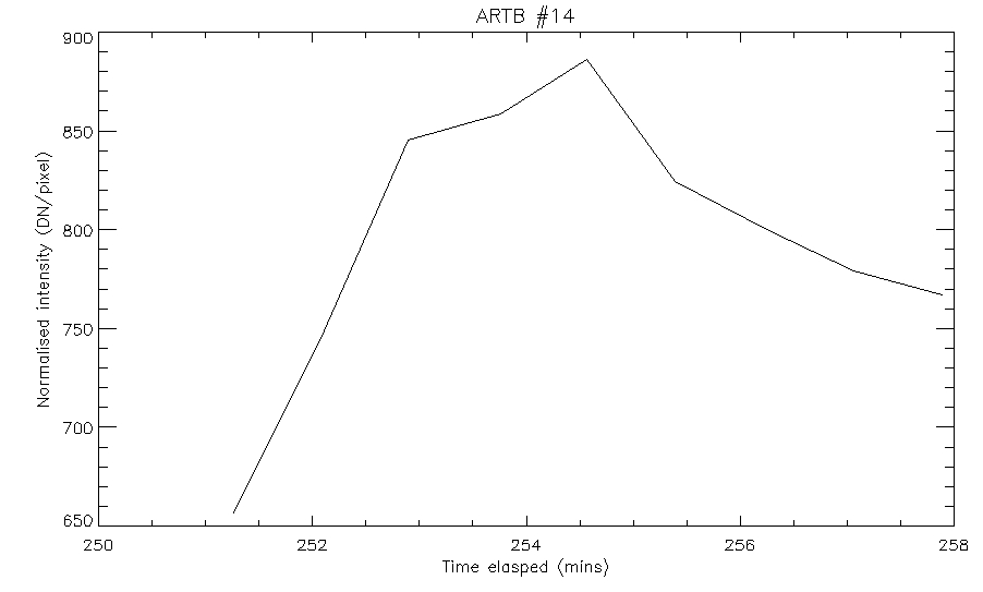
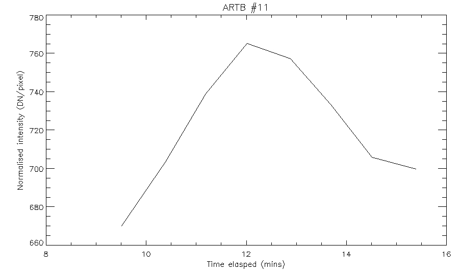
Run on ss_14: #1,2,9,11,13,14; ss_35: #1(?),8,12(?)Extracting ARTB Information
The 'find_artb' code that is used to search for ARTBs uses a binary counting system in order to record which ARTB lies where. As a default, each element in the image stack is set to -1; then, when a particular pixel is detected as being part of an ARTB, a value is added to that pixel. The value depends upon the ARTB number.
For example, an arbitrary pixel x would have value: x = -1+2^n, where n is the ARTB number, and the first few ARTBs would have pixels numbered as follows.
ARTB 1, i.e. n=1: x = -1+2^1=1ARTB 2, i.e. n=2: x = -1+2^2=3
ARTB 3, i.e. n=3: x = -1+2^3=7
ARTB 4, i.e. n=4: x = -1+2^4=15
:
ARTB 15, i.e. n=15: x = -1+2^15=32767
This counting method led to a problem however: the maximum size of an integer in IDL is 32767, which means that when the code attempts to calculate 2^16, it loops round and starts counting from upwards from -32768. As a result, it is not possible to record any more than 15 ARTBs in any one data set using this method.
There were two options at this point: either use another data type which can store larger integers, or chop the data sets up further so that no more than 15 were within an individual data set. We attempted to alter the code to use another data type, however this didn't work; therefore the only option was to chop up the data further before running the artb search code.
Making Light Curves
After running the code to find the ARTBs in each data set, the next step was to make a light curve for each one. The first step in doing this was to find the cross-section of the chosen ARTB. This was done by totalling 'artb_data' (the output of the ARTB search code) in the z-direction.


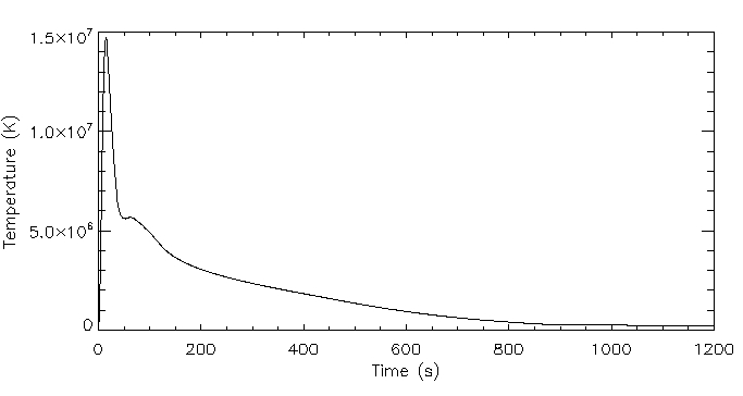
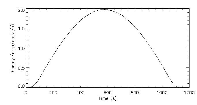
EBTEL Model

