At the end of the week I started running the simulation for the uniform area profile. All the simulations that I am running have the transition region placed at 0.25 with the thickness of 0.03. The mach number of the shock is 3.0.
We've run the simulation with non-uniform area profile. This profile shape looks similar to that of the transition region profile shape and has the form:
with R being "area ratio" (nrw), l0 "area position" (plc) and δ "area thickness" (thk). We've run the following set of simulations:
We analysed the data by looking at the movies created by the "tp_nondim" programme. Then we created 3 programs:
Due to the huge quantity of the output data from the above 3 programmes, we decided to calculate and plot:
As the number of these plots is so huge, I present here a sample of them which gives the sense of the distribution of the data.
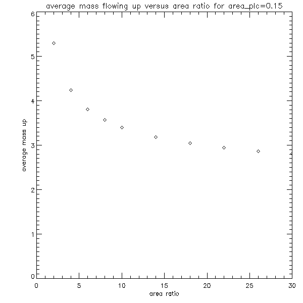
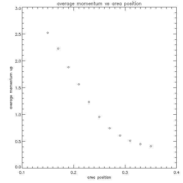
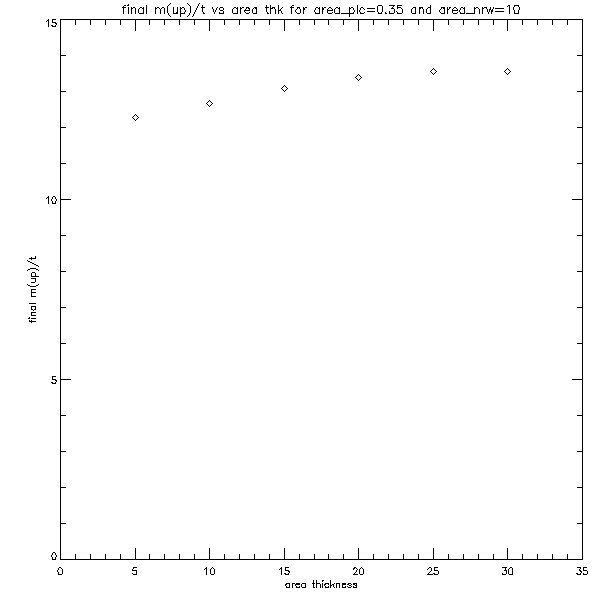
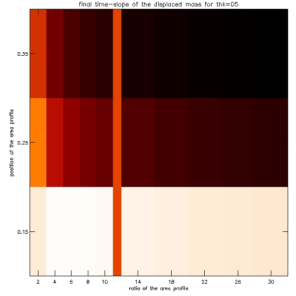
Because the number of these graphs is also very large, we decided to make density plots illustrating these results. The plots are shown below:
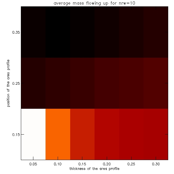
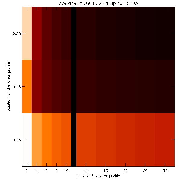
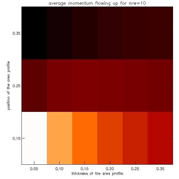
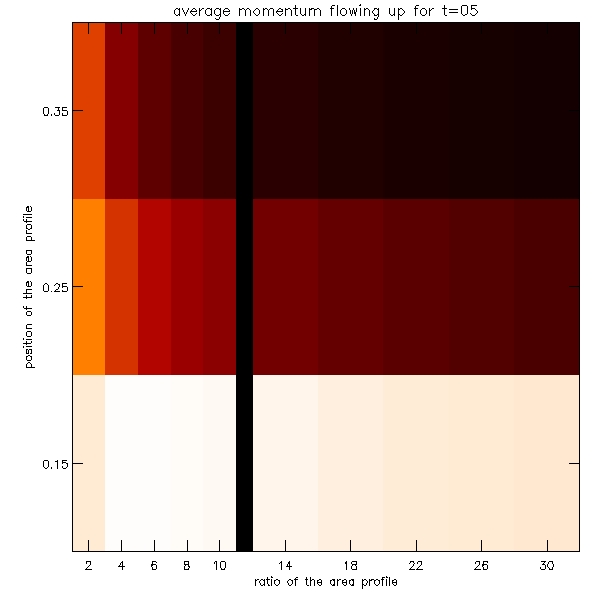
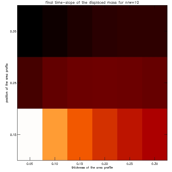
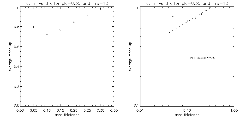
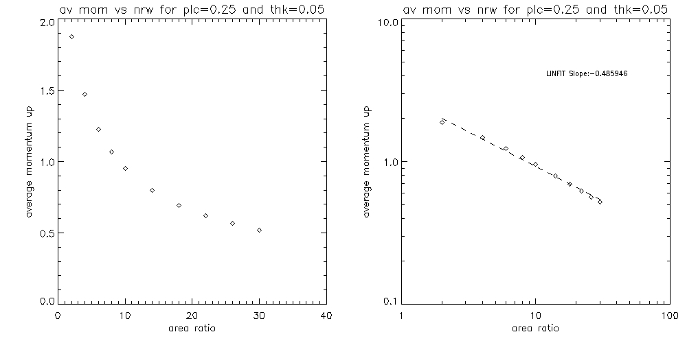
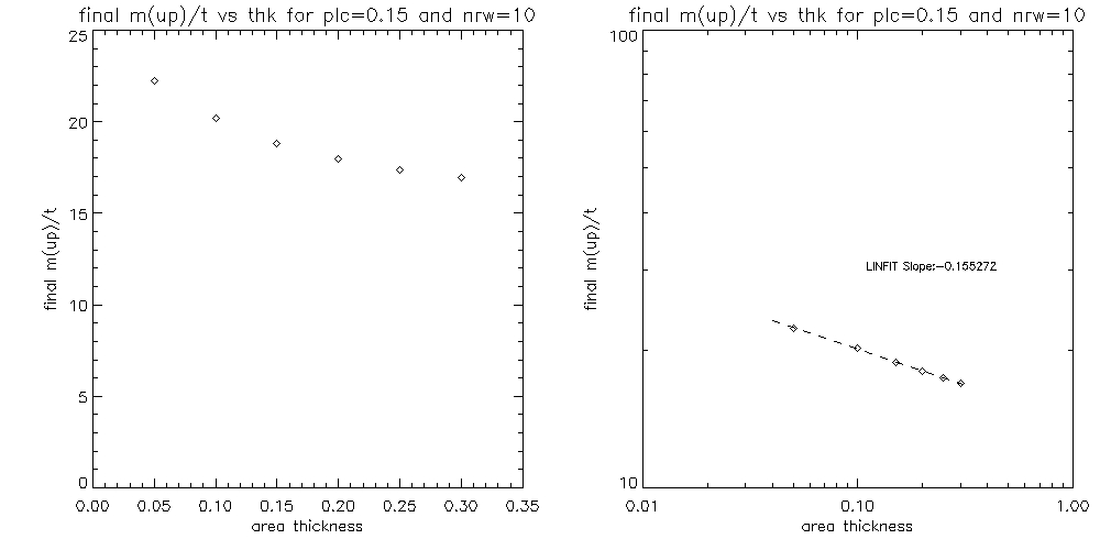
Since quite a few of the graphs shown above display a dependence which possibly can be modelled by a power law y=a*x^b, hence by plotting it on the log-log plot we would then expect to plot the function:
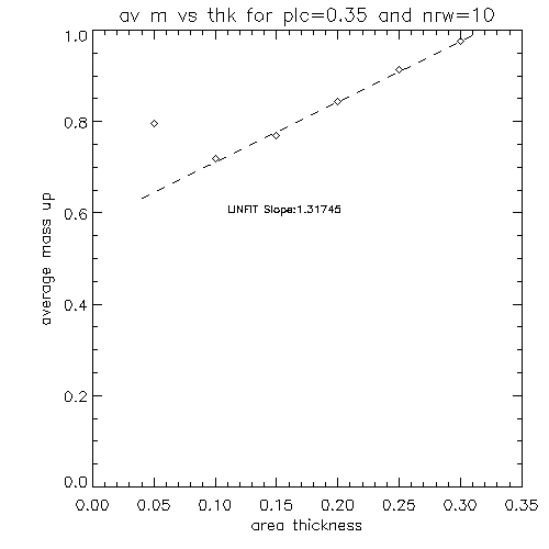
where b would be the slope of the graph. I plot below some of these fits on the log-log plot (for the first graph I exclude the point that stands out, which probably happens due to the fact that for this data point the area profile is above the transition region without any overlap between the two):
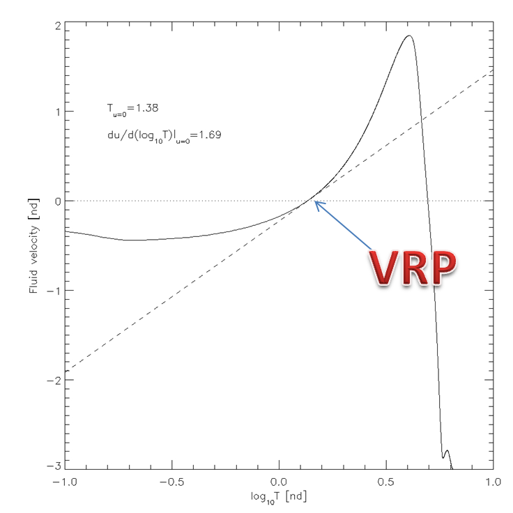
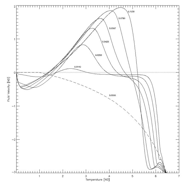
Due to the complexity of the problem we have decided to focus only on the significance of the position of the nozzle and keep the ratio and the thickness at the nozzle fixed, such that nrw=10 and thk=0.05. We focused on the evolution of the Velocity Reversal Point (VRP) which is the point where the velocity is equal to zero and which lies at the border of where the condensation region changes into the evaporation region. Below are 2 graphs, the first one is an example graph of Fluid Velocity vs Log(T) with VRP and the slope at VRP clearly marked. The second graph is a graph of Fluid Velocity vs Temperature in a uniform tube plotted for different time frames. Note that VRP tends to move down in T during early development of the evaporation.
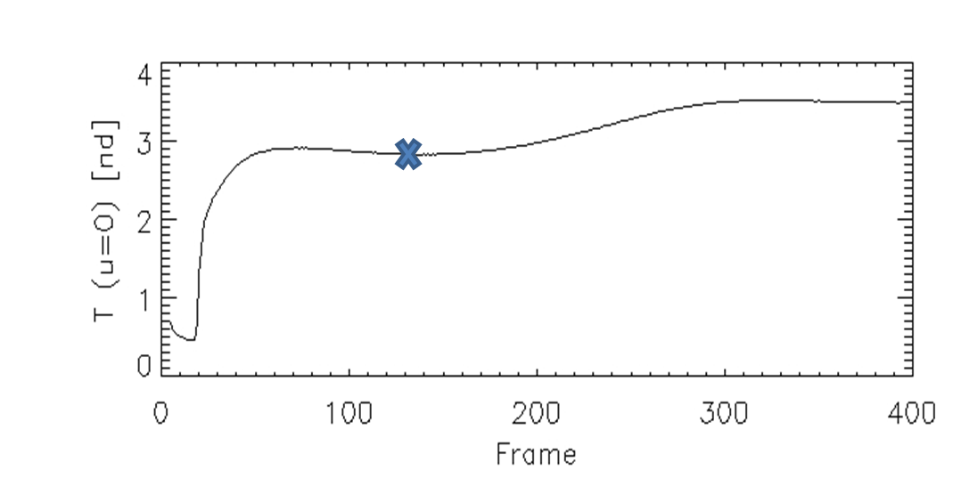
The temperature at the VRP changes over the time of the simulation. Hence we can plot this temperatue. The plot below is for plc=0.25. Note that there is a local minimum in T(u=0) between frames 130 and 150. We will call that time t0.
We can also plot the slope of the velocity vs logT graph at the VRP plotted as a function of time with the nozzle placed at 0.25.
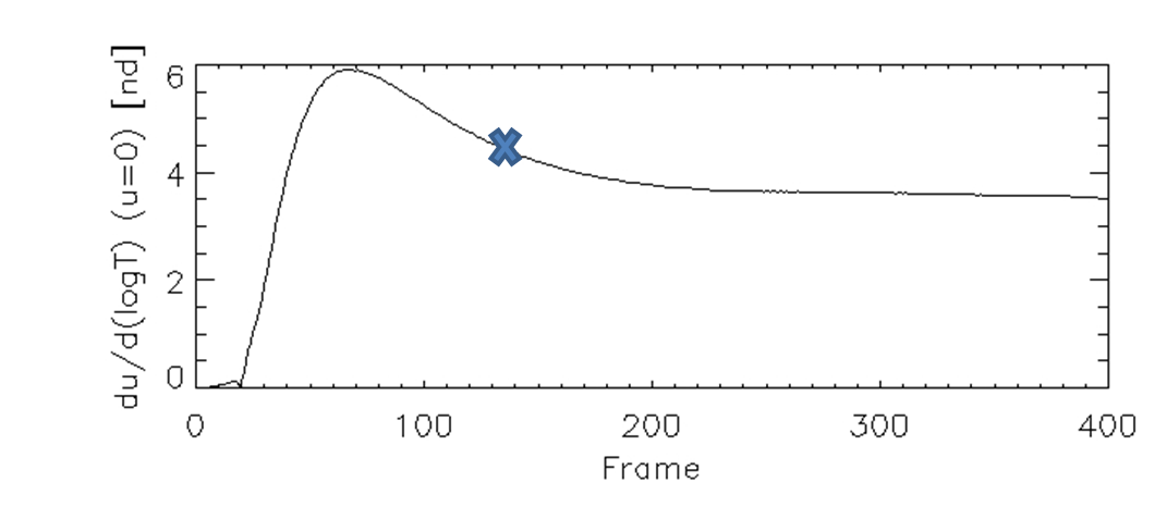
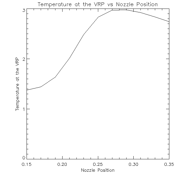
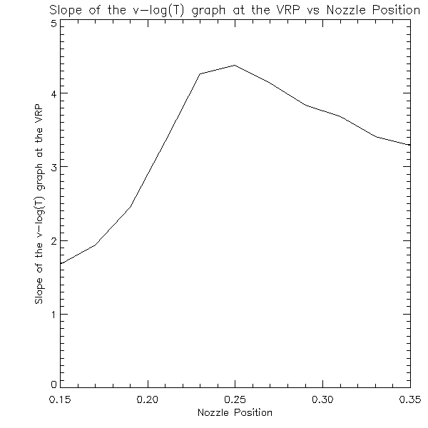
One can also find the time t0 for which the temperature at the Velocity Reversal Point is locally at its minimum (as marked on the previous graphs). We choose the minimum lying in the time interval for which the temperature doesn’t change rapidly with time, as that interval corresponds to what happens after the evaporation has already started. Then this minimum temperature and the slope on the velocity versus logT graph at the VRP at that time t0 are plotted as a function of the position of the nozzle.
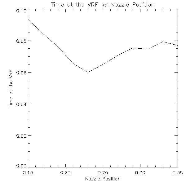
We can also plot time t0 as a function of the position of the nozzle.
At this stage, in order to look at the significance of the nozzle in an even more basic situation we investigated what happens to the thermal conduction front generated by the same shock, but this time propagating through the tube with no atmosphere at all (pressure, temperature and density are constant in the absence of the shock). We analysed the evolution of pressure, fluid velocity, density and temperature for three different area profiles: a)uniform, b)nozzle at 0.25 c)nozzle at 0.35. All three simulations have been overplotted on the same graphs. The movie can be seen under the link below:
Simulation for three different area profiles without atmosphereFrom all the four variables, temperature seems to be of greatest value to us, so we created the snapshots to show just the Temperature in this atmosphere-free shocktube.
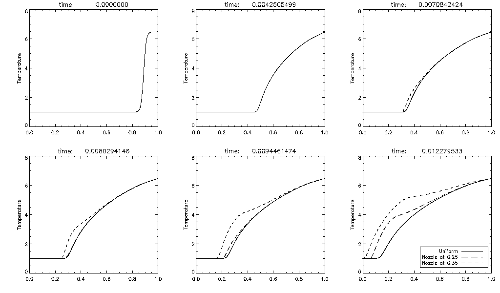
From these snapshots we can clearly see that TCF speeds up and the slope steepens at the front as it moves through the nozzle. The mathematical reason for this is as follows. We start with the energy equation for temperature:

We also have the following conditions for the atmosphere-free case

In 1D our derivatives become:

Hence the energy equation becomes:

Which can be rewritten as:
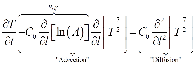
Hence we then conclude that normal diffusion is enhanced by effective thermal velocity ueff. The result of that is the steepening of the temperature gradient and acceleration of the TCF. However, the temperature and time at VRP vs position of the nozzle are not monotonic as we would expect from the above observations (temperature is not everywhere increasing and time is not everywhere decreasing). Hence this must be due to some additional effects of the atmosphere on the evaporation.
SPD Conference!
Since our form of the area-profile doesn't allow us to know exactly where the centre of the nozzle is (our equation defining the area profile is an equation for the logarithm of A rather than A, so plc is not exactly the position of the centre of the nozzle), we decided to change the area profile A(l) into a piecewise continuous function consisting of 3 straight lines:

We decided to investigate the moment when the evaporation firstly appears, that is when for the first time a positive velocity appears. We wanted to find the position and time of this first evaporation as well as the temperature at that moment and at that position. We decided to find those quantities for different positions of the nozzle. However, the very unexpected shape of the graphs of the temperature and time at the first evaporation vs nozzle position led Sean to the discovery that the heating term in the atmosphere programme didn't take into account the non-uniform tube profile. Hence after correcting that term we have re-run all the simulations with the piecewise function defining the shape of the nozzle.
Since we are interested only in the first part of the simulation, that is until the evaporation, we have created new runs which use the argument 'frmscl=0.1' in the evolver to make the frames 10 times denser, so that we have 10 times more frames and so we can say more accurately when the evaporation started. We created just the first 300 frames of this high resolution which covers the same duration as the original low resolution first 30 frames. Then we have again plotted position, time and temperature of the first evaporation as a function of nozzle position. The resulting graphs are shown below.
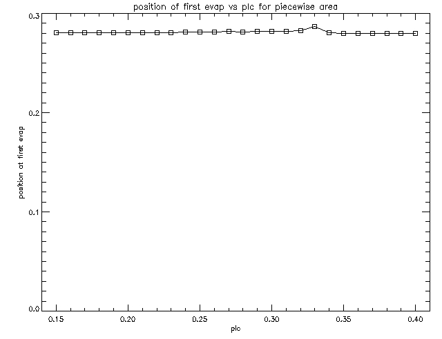
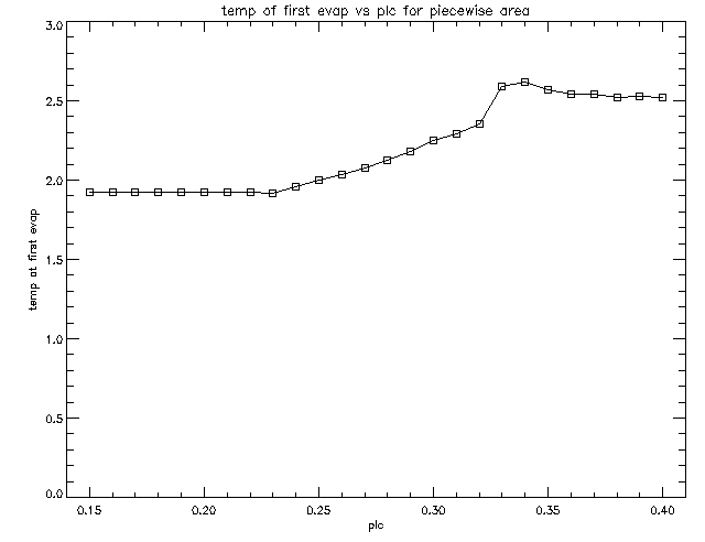
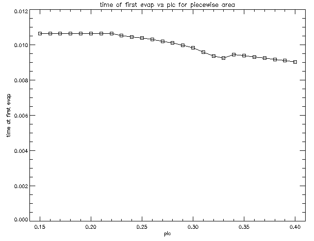
On those graphs we see that the evaporation starts at around l=0.28 no matter where the nozzle is placed (a slight exception is the case when plc=0.33). The reason for that is that l=0.28 is the front of the transition region. To understand the shape of the time and temperature graps, Sean proposed the following explanation:


In the case of our piecewise area profile, the above quantity is:

This function is a discontinuous function which is hyperbolically decreasing in the region where it is non-zero. It starts with the value of 90 at the bottom of the nozzle and falls down to 9 at the top of the nozzle. This explains the shape of the above graphs of temperature and time at the first evaporation. For the cases when the nozzle is places below 0.23, it doesn't affect the TCF before reaching transition region at 0.28 (this is where the evaporation starts). We see that the deeper into the nozzle the TCF can get before reaching transition region, the greater would be its advective speed. Moreover, for all cases when the TCF passes through the entire nozzle before reaching the TR, the TCF passes through the full region where the advective speed is non-zero which explains why on the right side of the graph showing the temperature of first evaporation our line is again flat.