Daily Log
06/05/2013
Hello World!
06/06/2013
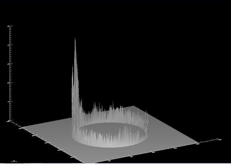
Today I created two programs that determine the intensities of n points in a radius specified by the user. The first program enebles the user to select an image from the solar dynamics observatory(instrument aia) taken in a specific moment in time. The second one has the same functionality with the only exception being that the image has to be provided by the user(It can be any image). The programs then surface and print the intensities with the corresponding coordinates. I also read some literature that presented some qualitive explanations of the "fuzzines" of the solar corona images taken in different euv bands. The filling-factor model being one of those possible explanations. Today I believe was the last day of pur IDL tutorials and it is quite possible that i will have to give a presentation of my programs tomorrow. Throughout the rest of the summer i will try to improve my created programs and utilize them to analyze the caracteristics of the solar corona and try to explain the "fuzzines" that surrounds them. I will also try to write in this log as time permits. Below is a sample shade surface from an sdo image taken on 2013/06/06 3:00:00 pm. The selected radius is 300 pixels and the chosen number of points was is 10000.

06/07/2013
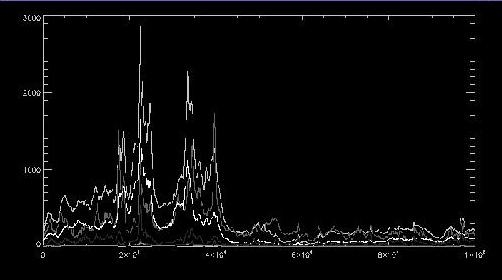
I just made a function that takes an image from each one of the different euv bands of aia and then performs the extract circle procedure on them. Below is an overlay plot of the intensities around a circle(same radius for all the images)(10000 points).For some odd reason the image refuses to look good when i upload it.

06/17/2013
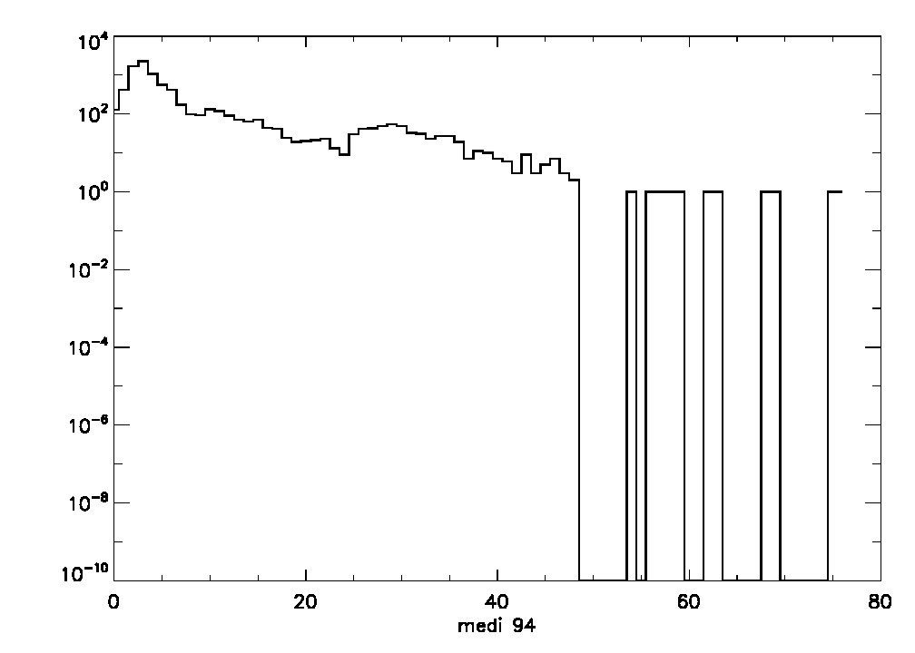
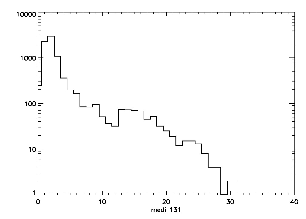
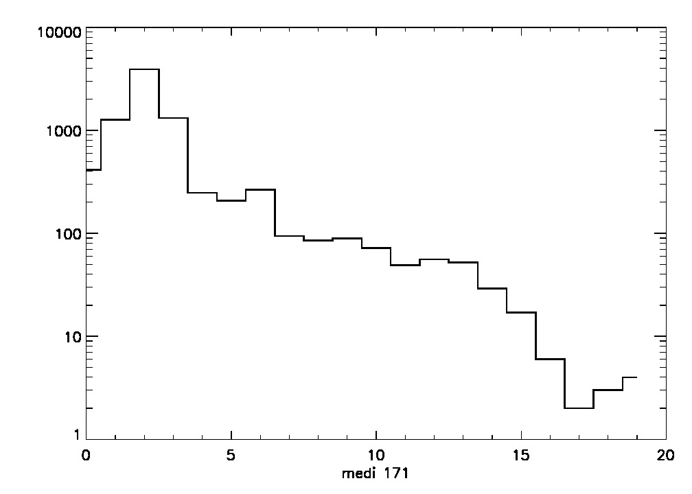
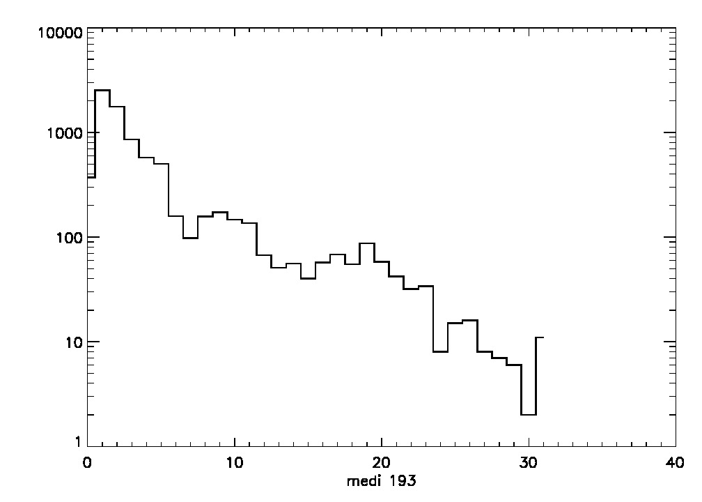
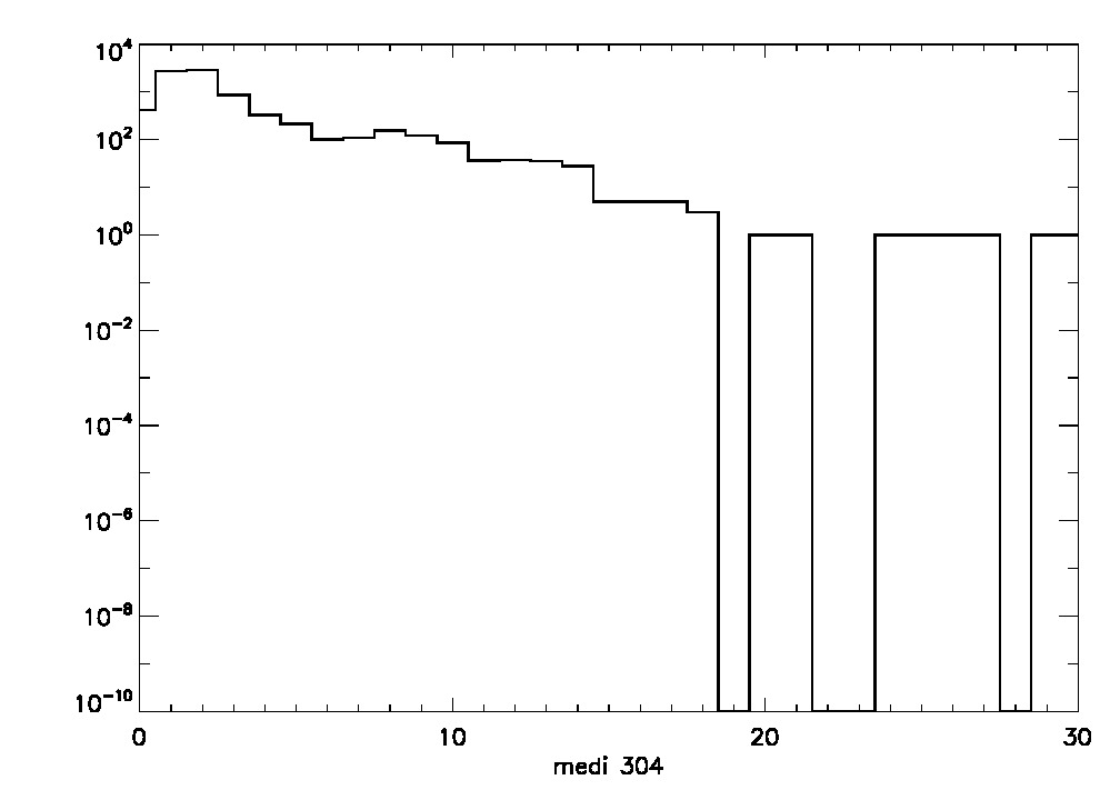
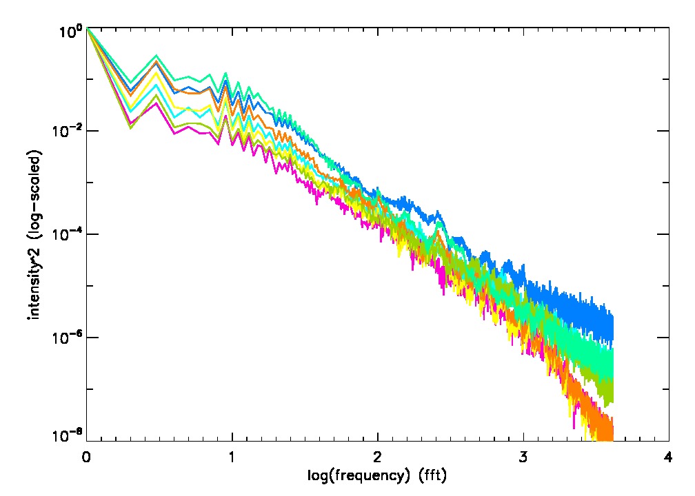
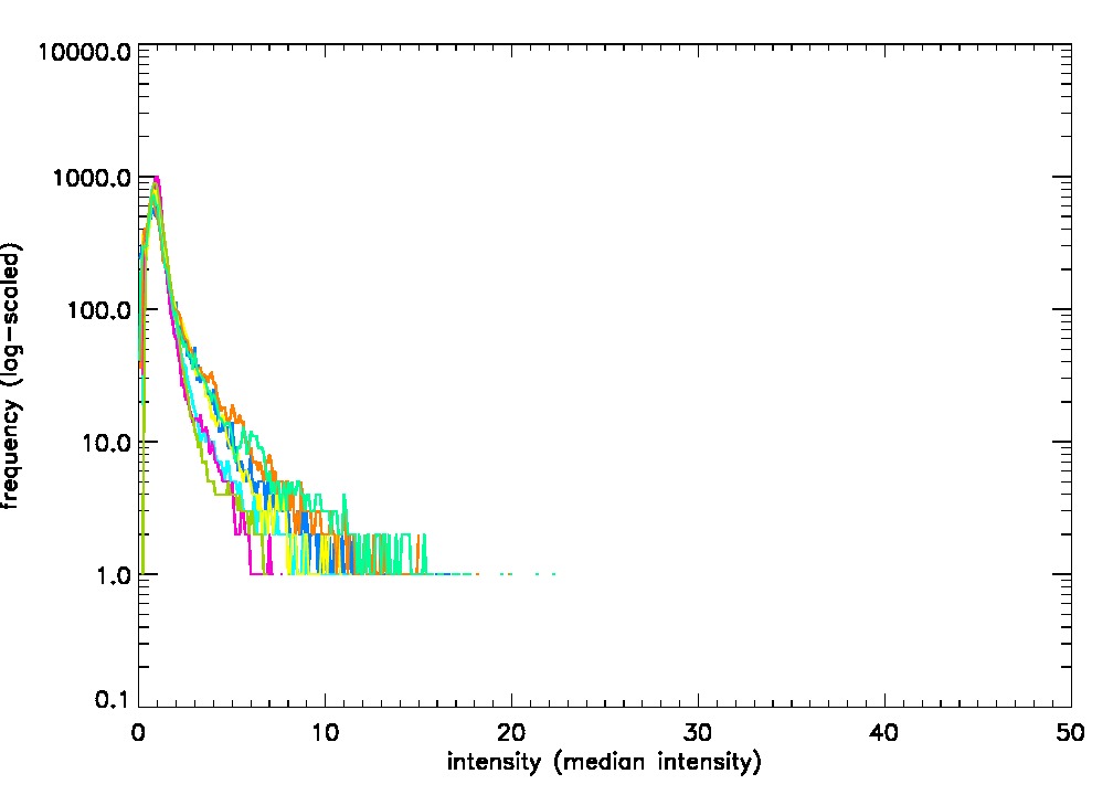
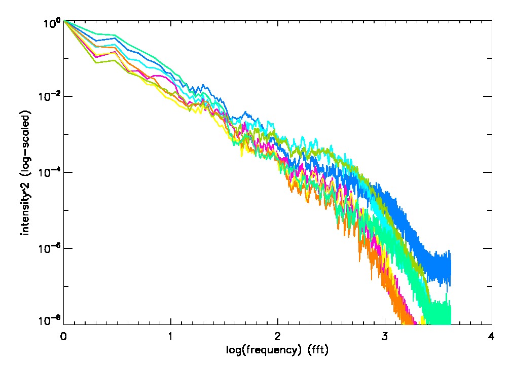
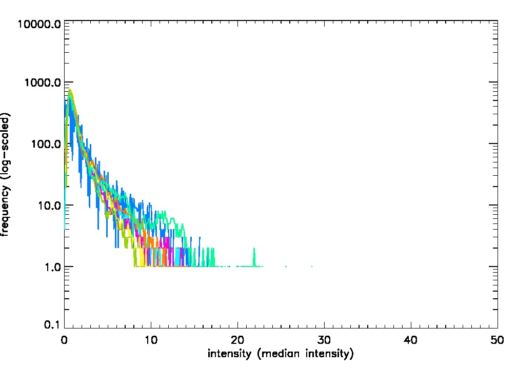
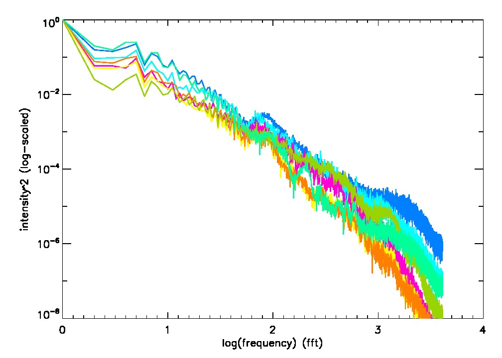
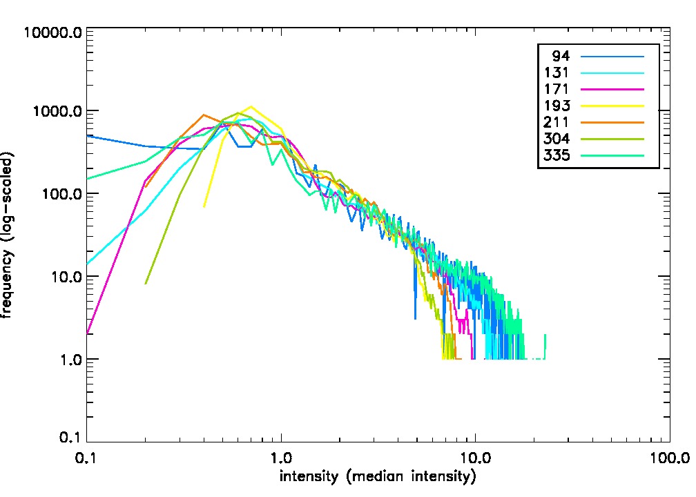
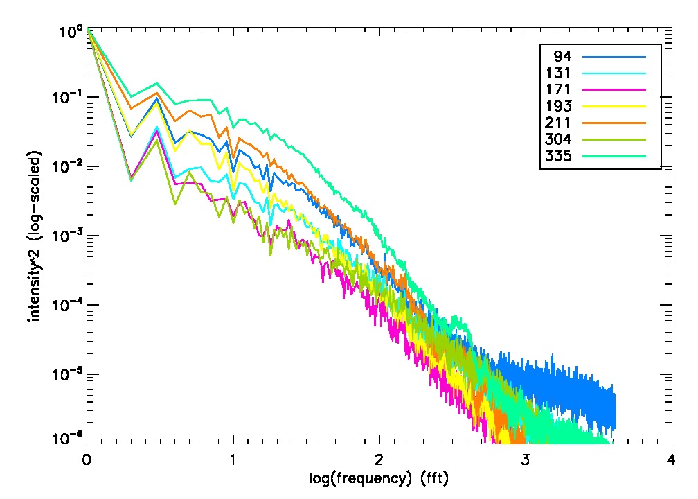
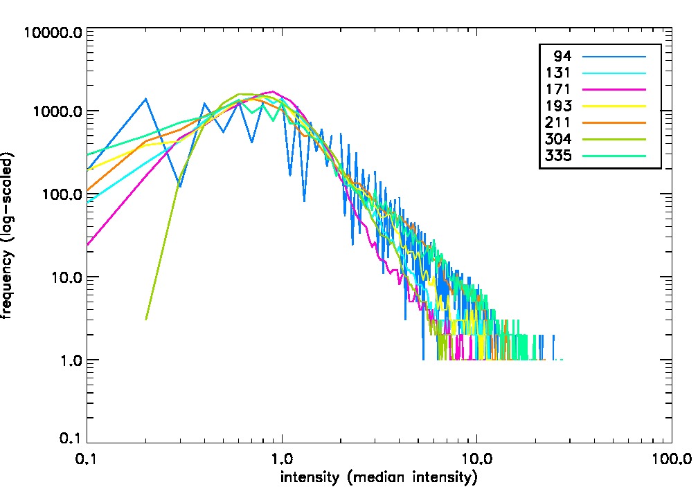
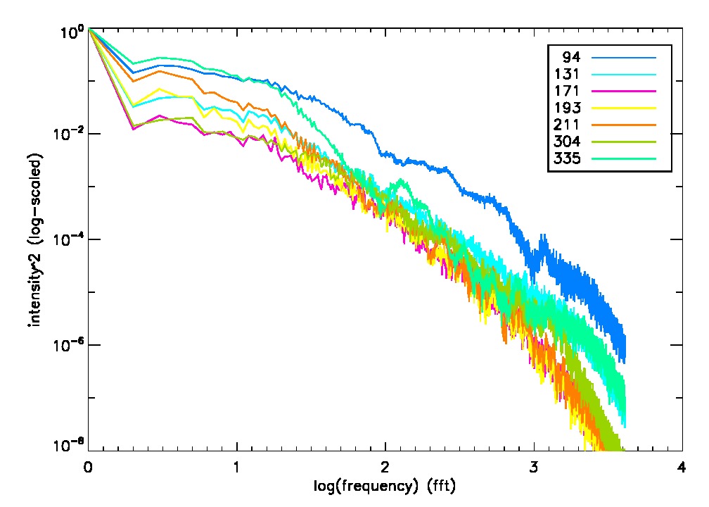
During these past days i improved my extract circle function to an extract anular region function that takes two radii r1 and r2 as arguments an allocates the mean intensities (r1-r2+1) points along the radial line to an index in a one-dimensional array. The array consists of n points where n is determined by the user. I also improved my code so it can take 5 AIA images from one pasbband and calculate the "mean" image. Then the extract anular region function can be used in the "mean" image to give a better representation of the solar corona structure along the region. I constructed quite a few histograms for the sake of making comparissons between the diffrent poassbands. Another comparisson technique that i used during last week (and i'm currently using right now) is performing a fast fourier transform on the obtained arrays. Below are a few images that illustrate some differences in the passbands.
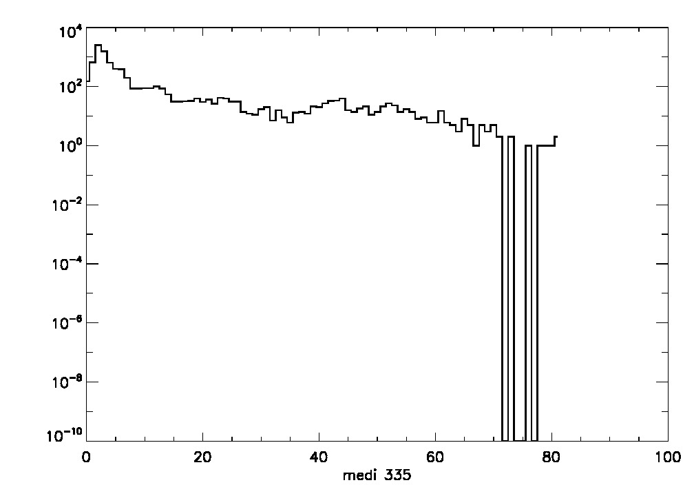
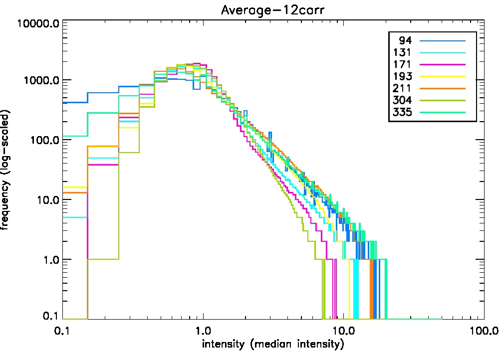
Frequency vs. Intensity in units of median intensity. The frequency axis is log scaled. (94/131/171/193/211/304/335 passbands 2013-01-01:2013-01-05 r:1610-1615)(images taken around 00:00:02)


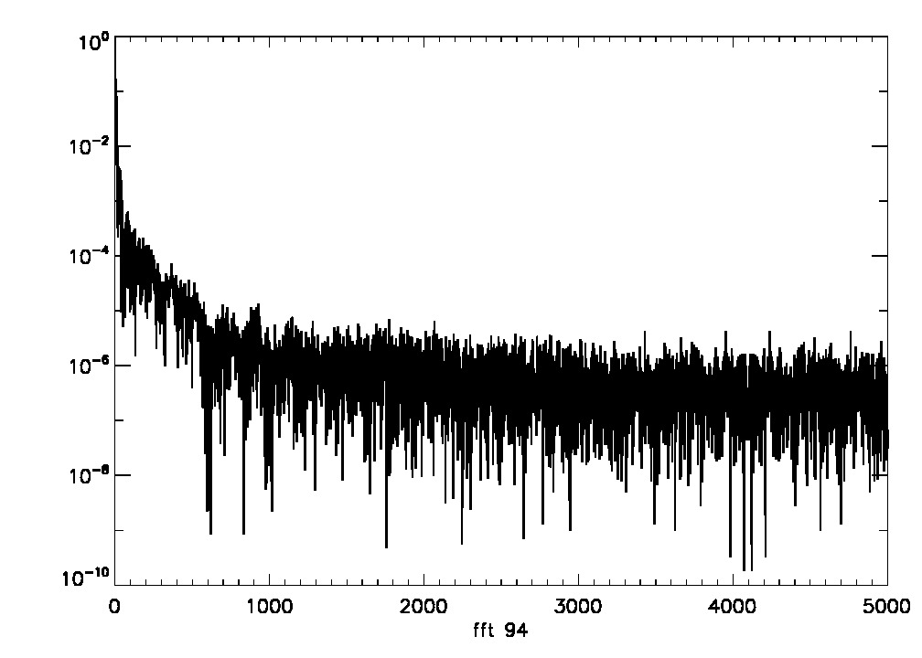
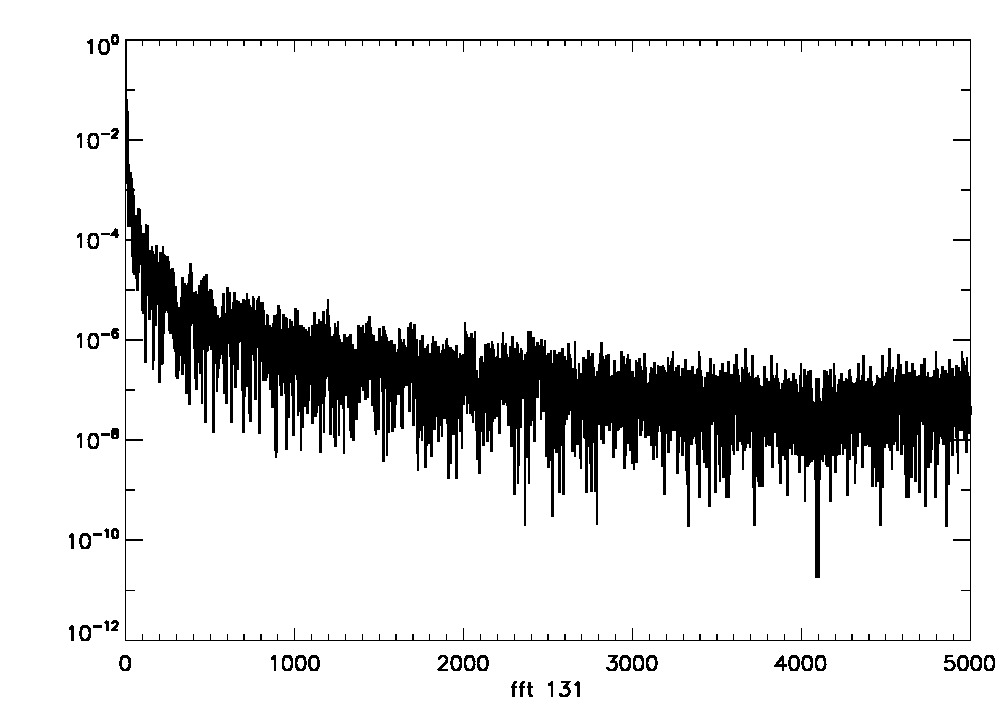
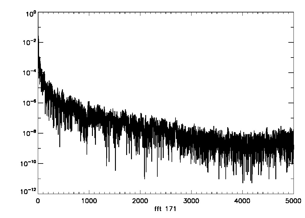
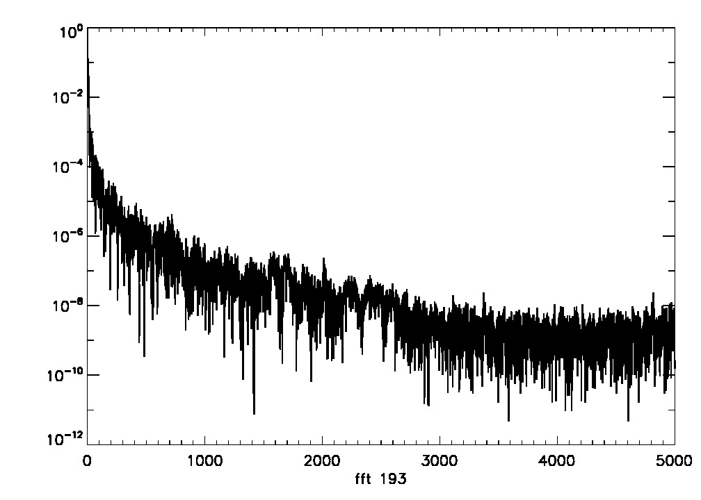
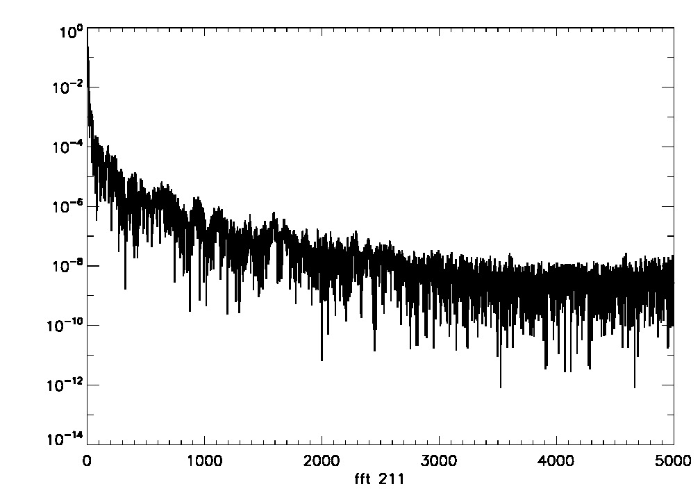
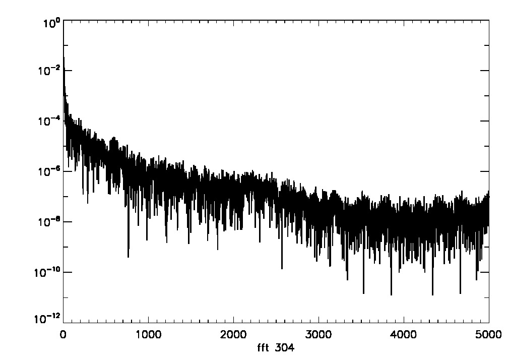
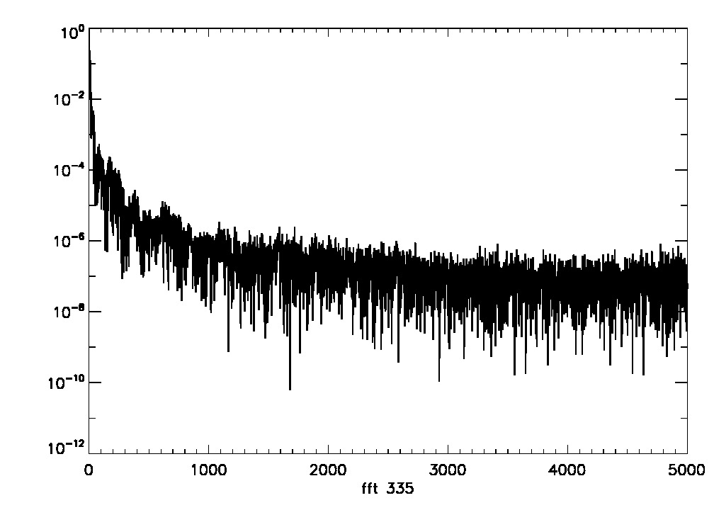
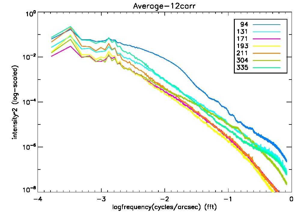
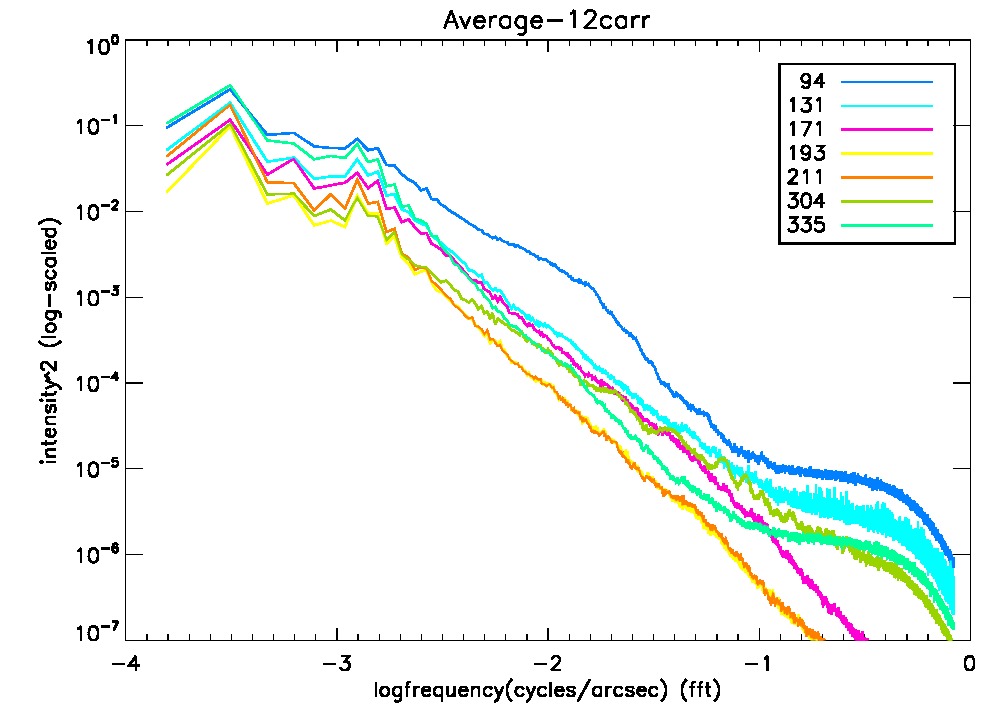
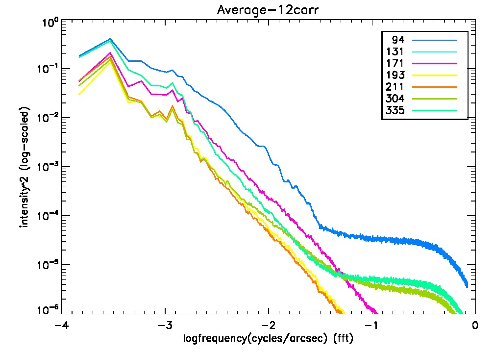
Plots of the fast fourier transforms of the same images used to make the last seven histograms. The y axis is log scaled.


06/19/2013
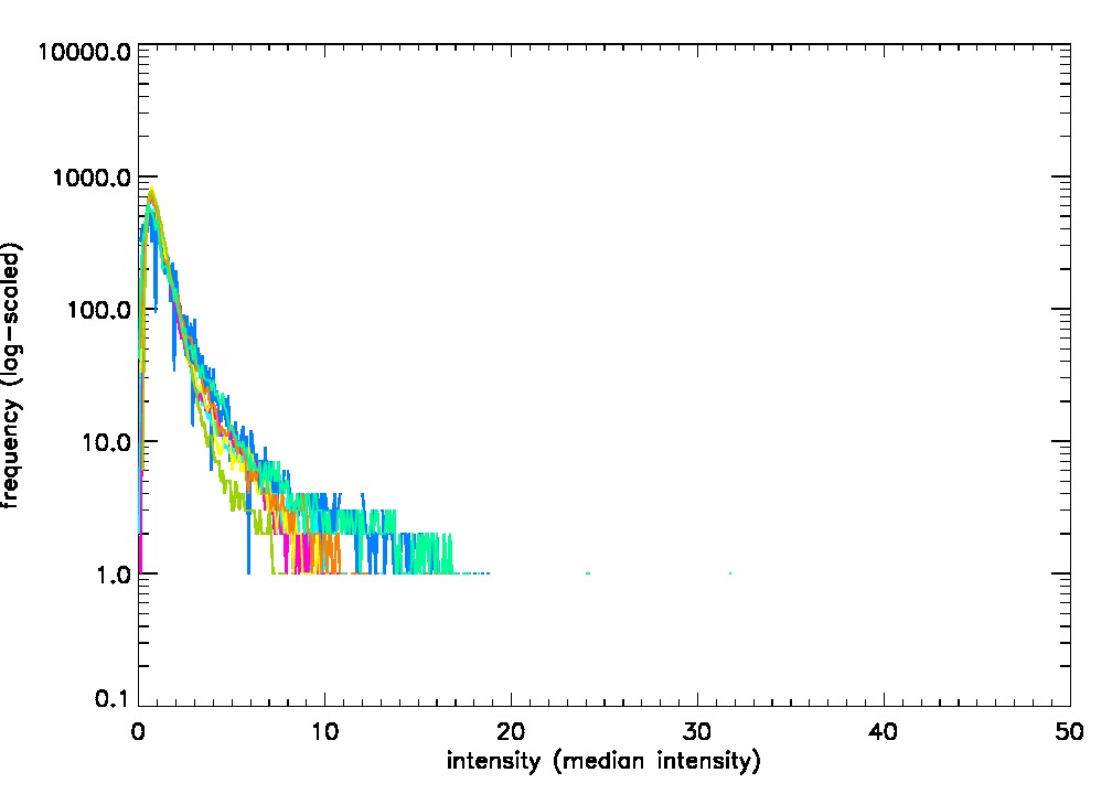
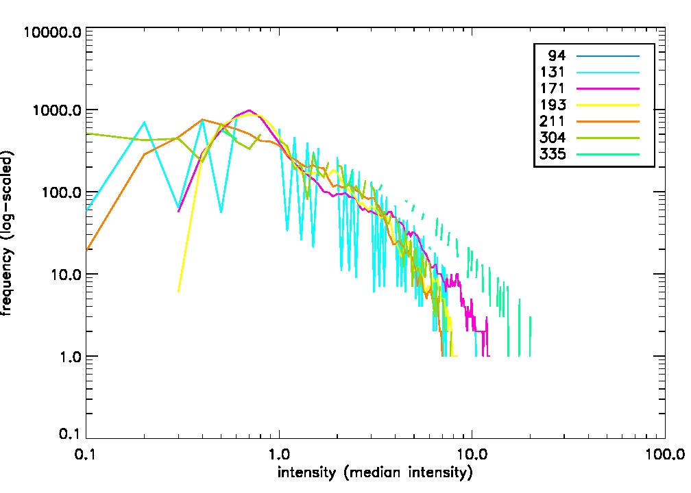
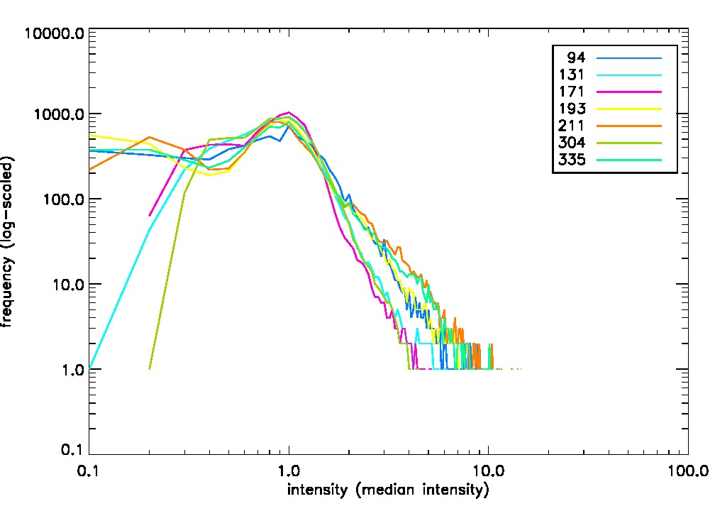
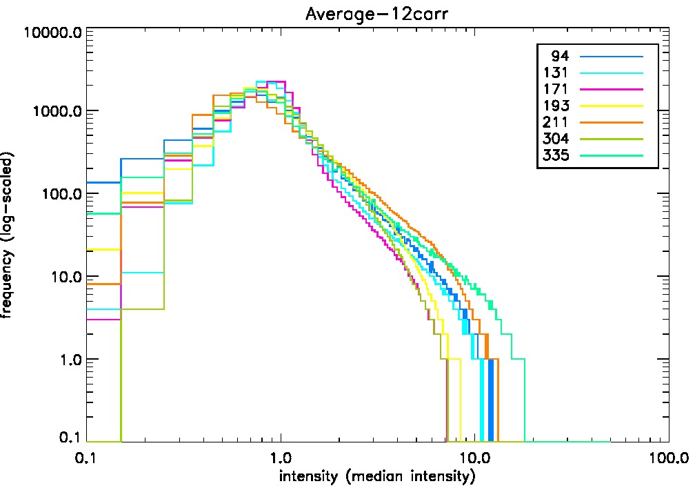
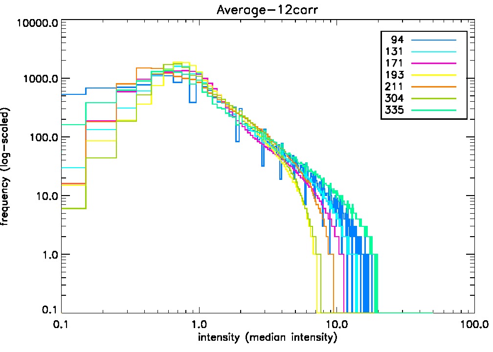
Today i created a program that constructs histograms and fourier transform plots using 12 one day apart images from each of the different AIA passbands. The program has to download 84 full resolution images so it takes quite some time to finish (the last run was a little more than 42mins 11.4322 secs). Below are the overlaid histogram and fft plots of 12 images taken from 2012-01-01 to 2012-01-12. All the images were taken at approximately 0:00:02 and the selected radii for the anular region were 1620 and 1625 pixels. For the fourier transform plot the original array was divided by the zero frequency component. We can observe that even though the overall structure of the plots are similar there are some visible differences. For example, we can observe that in the histogram plot the passbands that have a lower characteristic temperature fade quicker than the ones that possess a higher characteristic temperature. The latter ones have pixels whose intensity correspondes to roughly 15-25 times the value of the median intensity. I will run the program again with a different anular region selection (1500-1505) to determine if there are any noticeable differences.


The images below correspond to an anular region with r1=505 and r2=500.


The images below correspond to an anular region with r1=1005 and r2=1000


We can see from the histograms that the max intensities (units of median intensities) correspond principally to the 335,94 and 211 passbands, which would occupy the positions 3,2 and 4 respectively if we were to construct a list of all the AIA passband from highest to lowest characteristic temperature. The passband that has the highest characteristic temperature is 131 but it is important to note that the ions responsible for that are FeXX and FeXXIII and they are only present in solar flares. The plots, while not in perfect agreement, seem to show that the characteristic temperature of a waveband is correlated to the max intensity encountered in the histogram plots.
06/20/2013
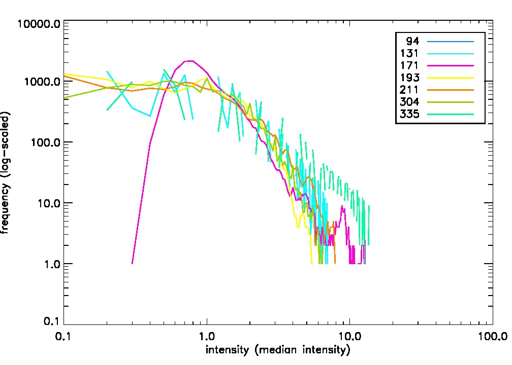
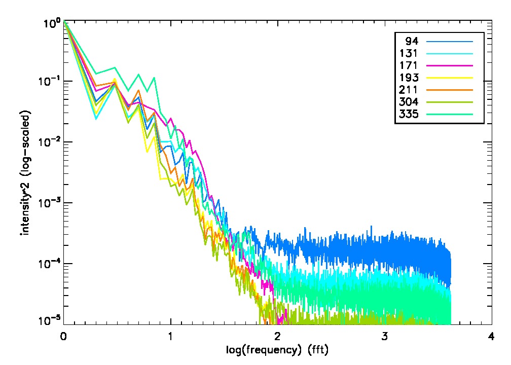
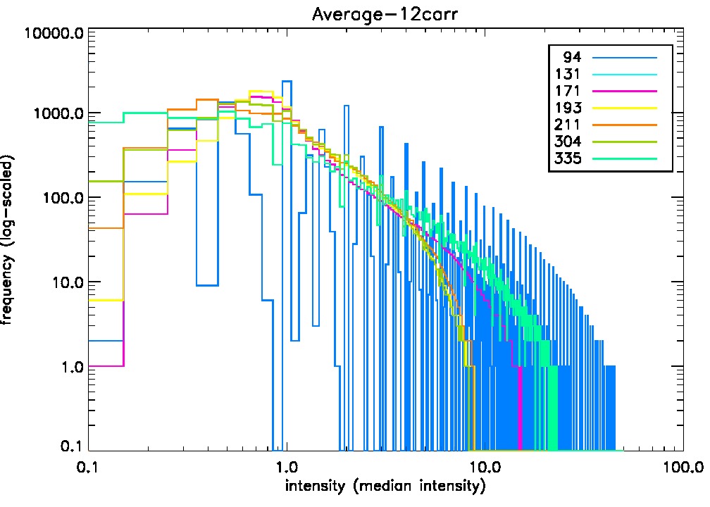
This will be a really short update about a result I obtained today. Tomorrow I will be presenting my results for the week in a little more depth. Today I tried using anular regions with the shorter radius bigger than the radius of the sun. There were some problems with the fourier transforms which I suspect are being caused by some negative intensity values close to the edges. The histogram plots look somewhat different to the plots using radii inside the sun. Below are three histogram plots for comparison. The first one corresponds to an anular region with radii 200/205, the second one to 1700/1705 and the last to 1900/1905. (The date for the images used is 2013-05-10:2013-05-21, each image was taken at approximately 0:00:02-0:00:03)


06/21/2013
During this week i have essentially been processing a bigger number of images. Everything is going pretty well except for some minor problems here and there. One of the problems that is bothering me at the moment is a "division by zero" that seems to be ocurring when I try to plot the fourier transforms of anular regions close to edges (not inside the visible radius of the sun). I also wrote a code to determine the 75 and 25 percentiles values of the intensities in an array from an anular region/circle. The results, so far, seem to be in agreement with my observations of max intensities in the 06/19/2013 entry. Just to give an example of the results here are the perecentile values for:
start:2011-01-01/aregion:1000-1005
94: 1.04/2.01
131: 1.01/1.49
171: 0.96/1.29
193: 1.00/1.60
211: 1.10/2.08
304: 1.02/1.36
335: 1.08/2.42
start:2013-05-10/aregion:1620-1625
94: 0.79/1.97
131: 0.84/2.04
171: 0.81/1.44
193: 0.76/1.79
211: 0.65/2.60
304: 0.78/1.99
335: 0.78/3.12
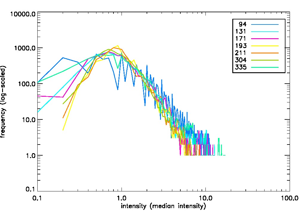
I have been using images from a random set of twelve consecutive day and analyzing 4 different anular regions (200-205, 500-505, 1000-1005, 1620-1625). I was reclutant at first to put legends in the plots but i guess they're much easier to read if i indeed allocate the legend inside the plotting area. I also log scaled the x axis for the histogram plot. Now it is much easier to see what happens with values close to the median intensity. I'm also going to start placing the start date for each plot as the plot title for clarity purposes. Below are some overlaid plot images I created today.

Histogram/aregion:1620-1625/2011-01-01

Fourier/aregion:1620-1625/2011-01-01

Histogram/aregion:1000-1005/2011-01-01

Fourier/aregion:1000-1005/2011-01-01

Histogram/aregion:1900-1905/2011-01-01

Fourier/aregion:1900-1905/2011-01-01
The last two images belong to an anular region of 1900-1905 and the code seemed to work fine. I guess this shows that the reason the code doesnt always work for r>1626 has something to do with the images themselves and not the code. Observing these plots we can see the disecrepancy between anular regions in the sun and anular regions outside the sun.
06/26/2013
Today i have been analizing data from 2013-06-01 -> 2013-06-12 and 2013-06-13 -> 2013-06-24. I changed the code for the intensity percentiles so that now the percentiles are computed and the averaged instead of the other way around. I also changed the frequency axis of the fft plots to cycles/arcsec units. Below are the intesity profiles of the studied sets of averaged images:
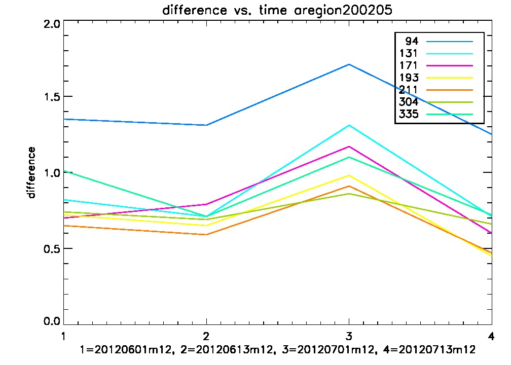
start:2012-06-01/aregion:200-205 start:2012-06-13/aregion:200-205
94: 0.54/1.89 difference: 1.35 94: 0.53/1.84 difference: 1.31
131: 0.70/1.53 difference: 0.82 131: 0.71/1.42 difference: 0.71
171: 0.73/1.43 difference: 0.70 171: 0.71/1.50 difference: 0.79
193: 0.75/1.47 difference: 0.72 193: 0.75/1.41 difference: 0.65
211: 0.73/1.78 difference: 0.65 211: 0.72/1.31 difference: 0.59
304: 0.71/1.45 difference: 0.74 304: 0.72/1.41 difference: 0.69
335: 0.64/1.65 difference: 1.01 335: 0.69/1.40 difference: 0.71
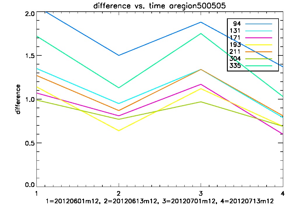
start:2012-06-01/aregion:500-505 start:2012-06-13/aregion:500-505
94: 0.44/2.50 difference: 2.06 94: 0.47/1.97 difference: 1.50
131: 0.65/2.00 difference: 1.35 131: 0.67/1.62 difference: 0.95
171: 0.65/1.72 difference: 1.07 171: 0.70/1.52 difference: 0.81
193: 0.66/1.74 difference: 1.09 193: 0.74/1.54 difference: 0.80
211: 0.65/1.92 difference: 1.27 211: 0.67/1.54 difference: 0.87
304: 0.68/1.67 difference: 0.99 304: 0.71/1.48 difference: 0.77
335: 0.58/2.30 difference: 1.72 335: 0.60/1.73 difference: 1.13
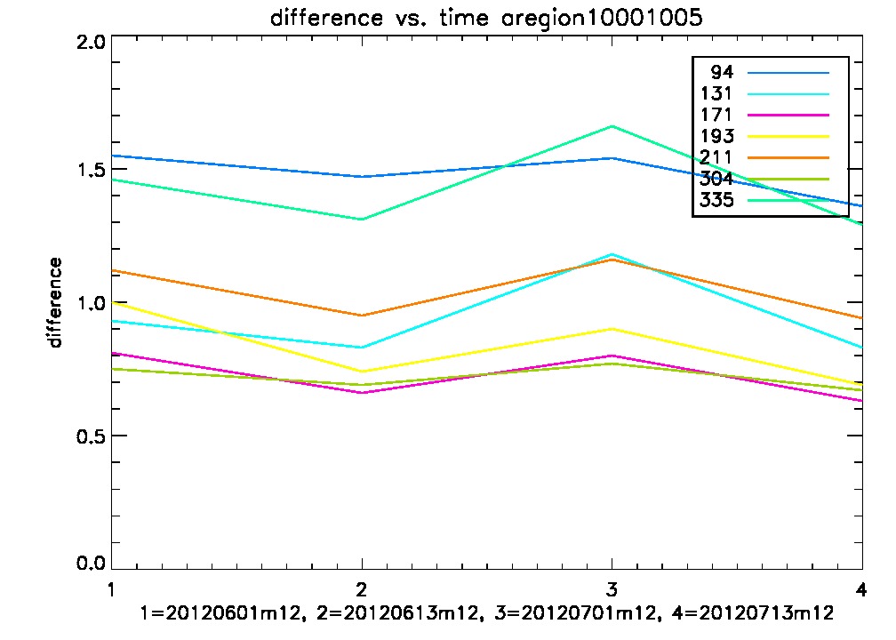
start:2012-06-01/aregion:1000-1005 start:2012-06-13/aregion:1000-1005
94: 0.47/2.02 difference: 1.55 94: 0.49/1.97 difference: 1.47
131: 0.68/1.61 difference: 0.93 131: 0.69/1.52 difference: 0.83
171: 0.71/1.52 difference: 0.81 171: 0.73/1.39 difference: 0.66
193: 0.68/1.67 difference: 1.00 193: 0.73/1.47 difference: 0.74
211: 0.69/1.80 difference: 1.12 211: 0.71/1.66 difference: 0.95
304: 0.71/1.46 difference: 0.75 304: 0.72/1.41 difference: 0.69
335: 0.62/2.08 difference: 1.46 335: 0.62/1.93 difference: 1.31
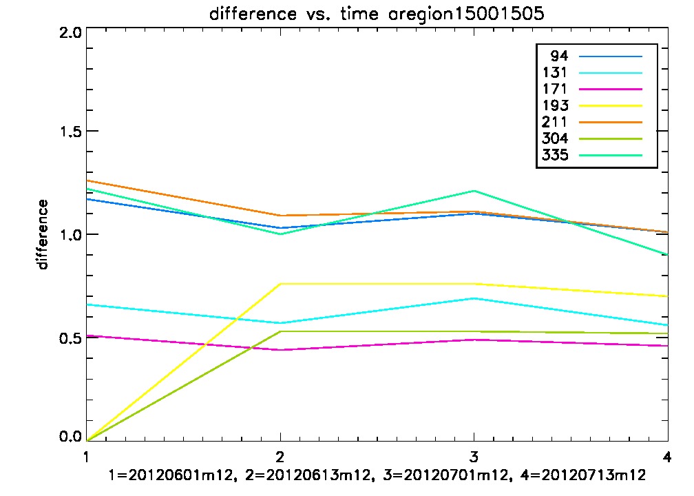
start:2012-06-01/aregion:1500-1505 start:2012-06-13/aregion:1500-1505
94: 0.59/1.76 difference: 1.17 94: 0.62/1.65 difference: 1.03
131: 0.75/1.41 difference: 0.66 131: 0.77/1.34 difference: 0.57
171: 0.79/1.30 difference: 0.51 171: 0.80/1.25 difference: 0.44
193: -7.20(?)/1.65 difference: 8.86(?) 193: 0.75/1.51 difference: 0.76
211: 0.69/1.95 difference: 1.26 211: 0.71/1.80 difference: 1.09
304: -61.8(?)/1.34 difference: 63.1(?) 304: 0.77/1.30 difference: 0.53
335: 0.69/1.92 difference: 1.22 335: 0.72/1.72 difference: 1.00
start:2012-06-01/aregion:1620-1625 start:2012-06-13/aregion:1620-1625
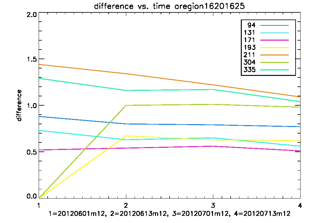
94: 0.68/1.56 difference: 0.88 94: 0.68/1.47 difference: 0.80
131: 0.79/1.51 difference: 0.73 131: 0.78/1.41 difference: 0.63
171: 0.78/1.31 difference: 0.52 171: 0.78/1.31 difference: 0.54
193: -3.16(?)/1.52 difference: 4.68(?) 193: 0.73/1.41 difference: 0.67
211: 0.63/2.08 difference: 1.44 211: 0.65/2.00 difference: 1.34
304: -237(?)/1.77 difference: 239(?) 304: 0.73/1.69 difference: 1.00
335: 0.71/2.00 difference: 1.29 335: 0.71/1.87 difference: 1.16
start:2012-06-01/aregion:1700-1705 start:2012-06-13/aregion:1700-1705
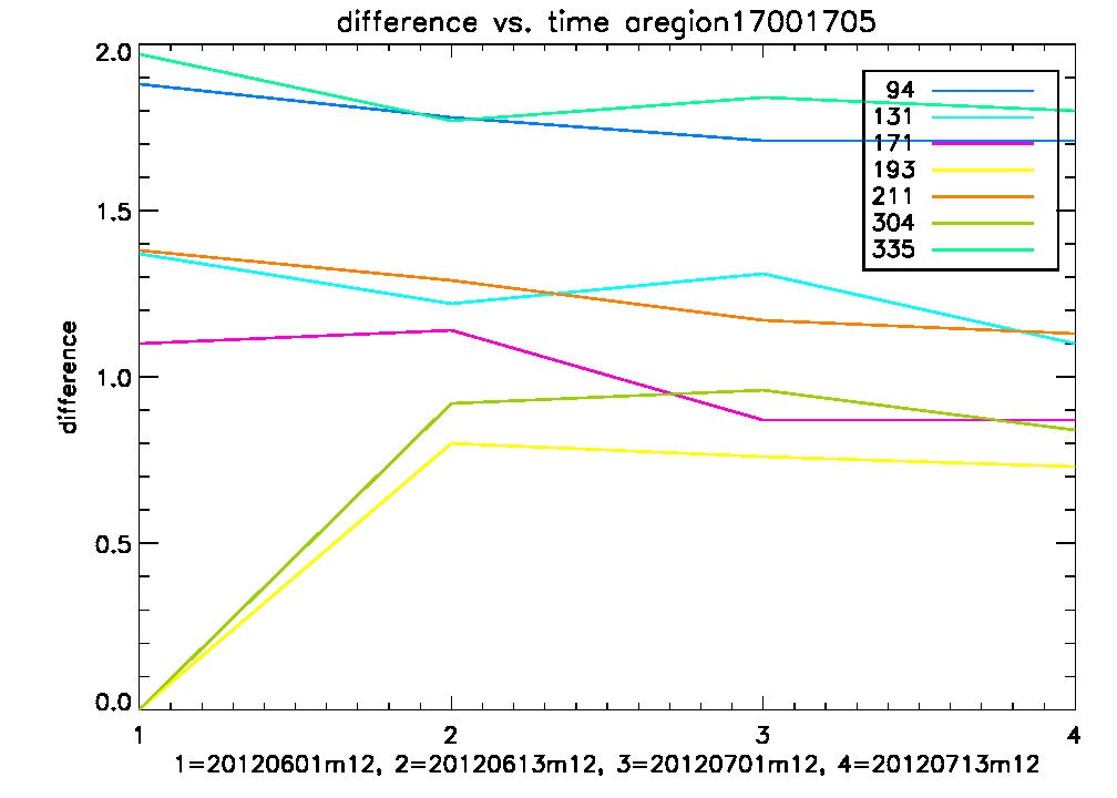
94: 0.46/2.35 difference: 1.88 94: 0.47/2.24 difference: 1.78
131: 0.65/2.01 difference: 1.37 131: 0.65/1.86 difference: 1.22
171: 0.72/1.83 difference: 1.10 171: 0.70/1.84 difference: 1.14
193: -8.04(?)/1.68 difference: 9.72(?) 193: 0.73/1.53 difference: 0.80
211: 0.61/1.99 difference: 1.38 211: 0.62/1.91 difference: 1.29
304: -511(?)/1.74 difference: 513(?) 304: 0.72/1.64 difference: 0.92
335: 0.57/2.54 difference: 1.97 335: 0.58/2.35 difference: 1.77
06/27/2013
start:2012-07-01/aregion:200-205 start:2012-07-13/aregion:200-205
94: 0.50/2.21 difference: 1.71 94: 0.48/1.73 difference: 1.25
131: 0.62/1.93 difference: 1.31 131: 0.70/1.41 difference: 0.71
171: 0.70/1.87 difference: 1.17 171: 0.76/1.36 difference: 0.60
193: 0.72/1.70 difference: 0.98 193: 0.82/1.28 difference: 0.45
211: 0.75/1.66 difference: 0.91 211: 0.80/1.28 difference: 0.47
304: 0.71/1.57 difference: 0.86 304: 0.73/1.39 difference: 0.66
335: 0.68/1.78 difference: 1.10 335: 0.68/1.40 difference: 0.72
start:2012-07-01/aregion:500-505 start:2012-07-13/aregion:500-505
94: 0.44/2.32 difference: 1.88 94: 0.51/1.89 difference: 1.37
131: 0.62/1.95 difference: 1.34 131: 0.69/1.47 difference: 0.79
171: 0.68/1.82 difference: 1.14 171: 0.73/1.38 difference: 0.64
193: 0.67/1.78 difference: 1.12 193: 0.76/1.45 difference: 0.69
211: 0.64/1.98 difference: 1.34 211: 0.72/1.53 difference: 0.81
304: 0.68/1.65 difference: 0.97 304: 0.72/1.41 difference: 0.69
335: 0.52/2.28 difference: 1.75 335: 0.62/1.65 difference: 1.03
start:2012-07-01/aregion:1000-1005 start:2012-07-13/aregion:1000-1005
94: 0.49/2.02 difference: 1.54 94: 0.48/1.84 difference: 1.36
131: 0.60/1.78 difference: 1.18 131: 0.68/1.51 difference: 0.83
171: 0.72/1.52 difference: 0.80 171: 0.75/1.38 difference: 0.63
193: 0.69/1.59 difference: 0.90 193: 0.75/1.44 difference: 0.69
211: 0.66/1.82 difference: 1.16 211: 0.72/1.66 difference: 0.94
304: 0.71/1.48 difference: 0.77 304: 0.73/1.39 difference: 0.67
335: 0.58/2.24 difference: 1.66 335: 0.63/1.92 difference: 1.29
start:2012-07-01/aregion:1500-1505 start:2012-07-13/aregion:1500-1505
94: 0.61/1.71 difference: 1.10 94: 0.61/1.61 difference: 1.01
131: 0.72/1.40 difference: 0.69 131: 0.77/1.33 difference: 0.56
171: 0.78/1.27 difference: 0.49 171: 0.79/1.25 difference: 0.46
193: 0.76/1.52 difference: 0.76 193: 0.75/1.45 difference: 0.70
211: 0.73/1.83 difference: 1.11 211: 0.69/1.70 difference: 1.01
304: 0.78/1.31 difference: 0.53 304: 0.78/1.30 difference: 0.52
335: 0.70/1.91 difference: 1.21 335: 0.72/1.62 difference: 0.90
start:2012-07-01/aregion:1620-1625 start:2012-07-13/aregion:1620-1625
94: 0.69/1.48 difference: 0.79 94: 0.69/1.46 difference: 0.77
131: 0.75/1.40 difference: 0.65 131: 0.79/1.35 difference: 0.56
171: 0.76/1.32 difference: 0.56 171: 0.77/1.29 difference: 0.51
193: 0.75/1.38 difference: 0.63 193: 0.75/1.37 difference: 0.62
211: 0.67/1.89 difference: 1.22 211: 0.65/1.73 difference: 1.09
304: 0.71/1.71 difference: 1.01 304: 0.73/1.71 difference: 0.98
335: 0.71/1.87 difference: 1.17 335: 0.70/1.73 difference: 1.04
start:2012-07-01/aregion:1700-1705 start:2012-07-13/aregion:1700-1705
94: 0.47/2.18 difference: 1.71 94: 0.43/2.14 difference: 1.71
131: 0.60/1.91 difference: 1.31 131: 0.67/1.77 difference: 1.10
171: 0.71/1.58 difference: 0.87 171: 0.73/1.59 difference: 0.87
193: 0.75/1.51 difference: 0.76 193: 0.75/1.48 difference: 0.73
211: 0.64/1.81 difference: 1.17 211: 0.62/1.75 difference: 1.13
304: 0.70/1.66 difference: 0.96 304: 0.74/1.57 difference: 0.84
335: 0.59/2.44 difference: 1.84 335: 0.58/2.38 difference: 1.80
06/28/2013
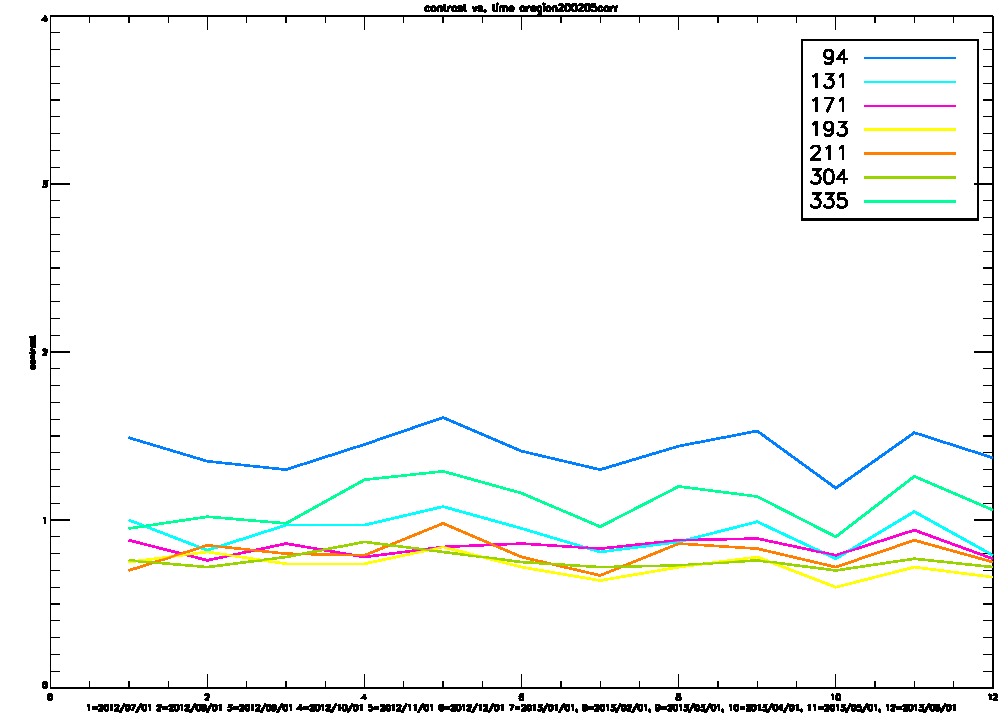
Today i added some data to the past two entries. I also created some difference vs. time plots of said data. The plots can be seen below:


07/01/2013
start:2012-08-01/aregion:200-205 start:2012-08-13/aregion:200-205
94: 0.46/1.80 difference: 1.34 94: 0.45/1.76 difference: 1.32
131: 0.68/1.50 difference: 0.82 131: 0.71/1.50 difference: 0.79
171: 0.70/1.49 difference: 0.79 171: 0.75/1.45 difference: 0.70
193: 0.76/1.59 difference: 0.83 193: 0.71/1.40 difference: 0.68
211: 0.73/1.61 difference: 0.88 211: 0.68/1.48 difference: 0.81
304: 0.71/1.41 difference: 0.70 304: 0.72/1.44 difference: 0.72
335: 0.67/1.72 difference: 1.05 335: 0.63/1.67 difference: 1.04
start:2012-08-01/aregion:500-505 start:2012-08-13/aregion:500-505
94: 0.48/2.16 difference: 1.68 94: 0.48/1.79 difference: 1.31
131: 0.65/1.74 difference: 1.08 131: 0.69/1.50 difference: 0.81
171: 0.66/1.70 difference: 1.04 171: 0.71/1.41 difference: 0.70
193: 0.69/1.68 difference: 0.99 193: 0.74/1.42 difference: 0.68
211: 0.68/1.73 difference: 1.05 211: 0.71/1.47 difference: 0.76
304: 0.69/1.53 difference: 0.84 304: 0.70/1.49 difference: 0.79
335: 0.62/1.79 difference: 1.17 335: 0.59/1.67 difference: 1.08
start:2012-08-01/aregion:1000-1005 start:2012-08-13/aregion:1000-1005
94: 0.49/2.16 difference: 1.68 94: 0.48/1.75 difference: 1.27
131: 0.66/1.81 difference: 1.15 131: 0.70/1.45 difference: 0.75
171: 0.68/1.63 difference: 0.95 171: 0.72/1.36 difference: 0.64
193: 0.69/1.68 difference: 0.99 193: 0.76/1.41 difference: 0.65
211: 0.64/1.92 difference: 1.28 211: 0.72/1.58 difference: 0.86
304: 0.70/1.49 difference: 0.79 304: 0.73/1.38 difference: 0.65
335: 0.58/2.33 difference: 1.76 335: 0.64/1.65 difference: 1.00
start:2012-08-01/aregion:1500-1505 start:2012-08-13/aregion:1500-1505
94: 0.62/1.67 difference: 1.05 94: 0.62/1.59 difference: 0.97
131: 0.76/1.37 difference: 0.61 131: 0.77/1.34 difference: 0.57
171: 0.78/1.27 difference: 0.50 171: 0.77/1.24 difference: 0.46
193: 0.74/1.52 difference: 0.78 193: 0.76/1.48 difference: 0.72
211: 0.69/1.73 difference: 1.03 211: 0.71/1.74 difference: 1.03
304: 0.78/1.32 difference: 0.55 304: 0.78/1.32 difference: 0.53
335: 0.67/1.71 difference: 1.04 335: 0.71/1.64 difference: 0.93
start:2012-08-01/aregion:1620-1625 start:2012-08-13/aregion:1620-1625
94: 0.69/1.53 difference: 0.84 94: 0.70/1.45 difference: 0.75
131: 0.80/1.46 difference: 0.66 131: 0.81/1.37 difference: 0.56
171: 0.76/1.29 difference: 0.53 171: 0.77/1.28 difference: 0.51
193: 0.74/1.43 difference: 0.69 193: 0.76/1.42 difference: 0.66
211: 0.62/1.82 difference: 1.20 211: 0.64/1.93 difference: 1.30
304: 0.72/1.67 difference: 0.95 304: 0.72/1.69 difference: 0.97
335: 0.69/1.82 difference: 1.13 335: 0.71/1.76 difference: 1.05
start:2012-08-01/aregion:1700-1705 start:2012-08-13/aregion:1700-1705
94: 0.48/2.13 difference: 1.65 94: 0.46/1.94 difference: 1.48
131: 0.69/1.92 difference: 1.23 131: 0.69/1.72 difference: 1.03
171: 0.73/1.76 difference: 1.02 171: 0.71/1.51 difference: 0.80
193: 0.77/1.57 difference: 0.80 193: 0.77/1.51 difference: 0.74
211: 0.59/1.78 difference: 1.19 211: 0.60/1.77 difference: 1.17
304: 0.72/1.60 difference: 0.88 304: 0.72/1.58 difference: 0.87
335: 0.58/2.42 difference: 1.84 335: 0.58/2.30 difference: 1.73
07/17/2013
I am analyzing data corresponding to roughly a full carrington rotation of sun. The complete results should be available for comparisson with past results by tomorrow.
07/17/2013
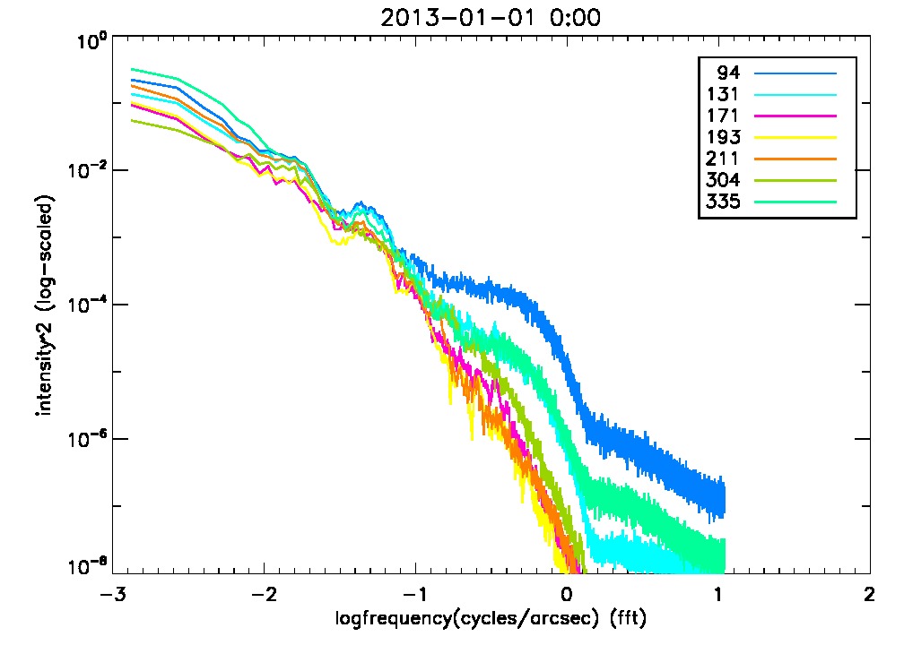
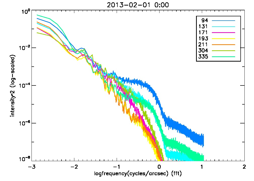
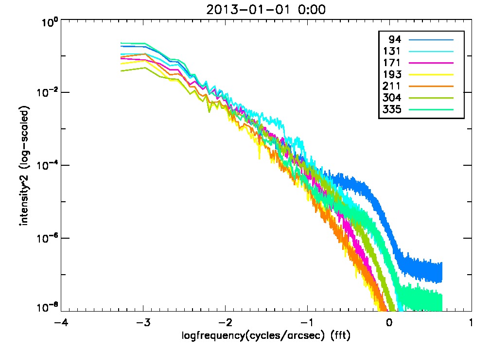
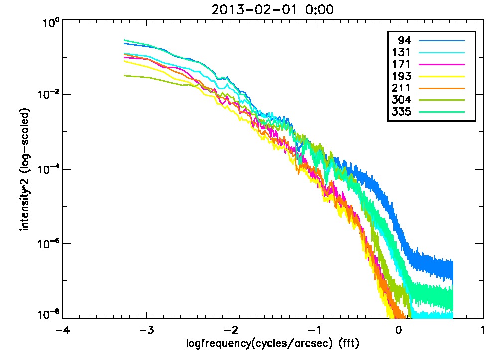
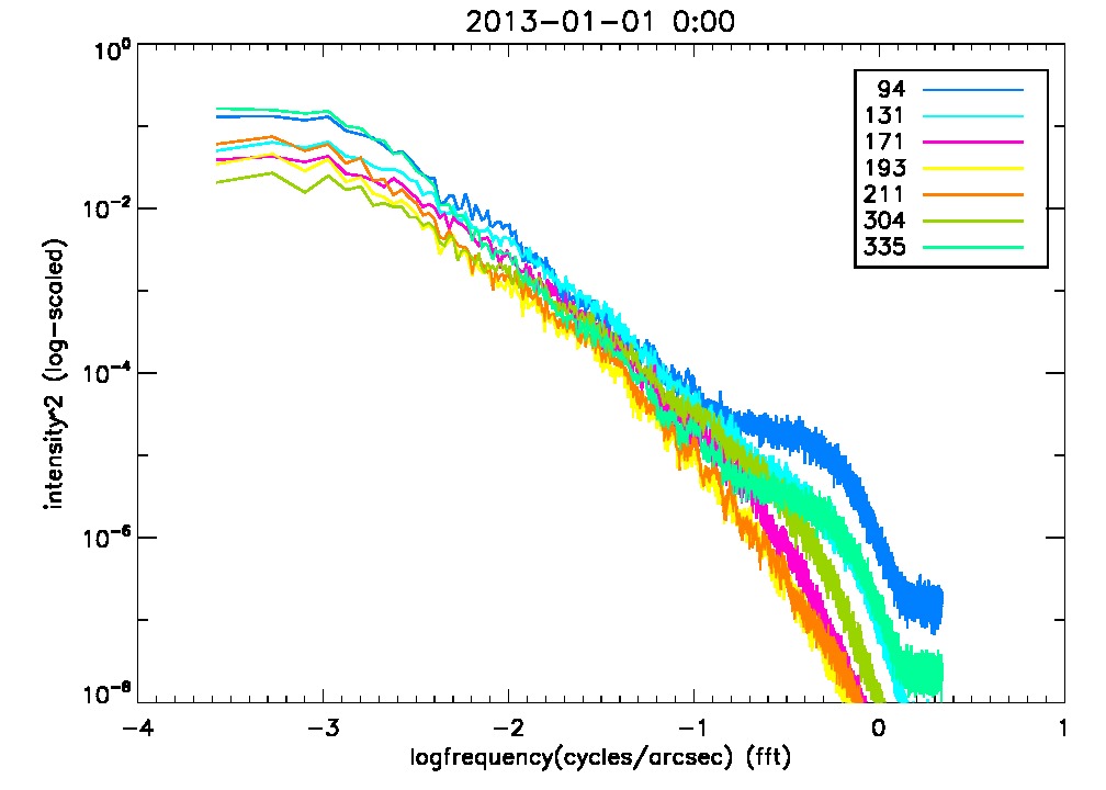
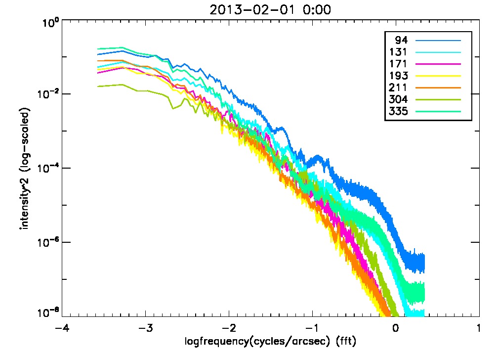
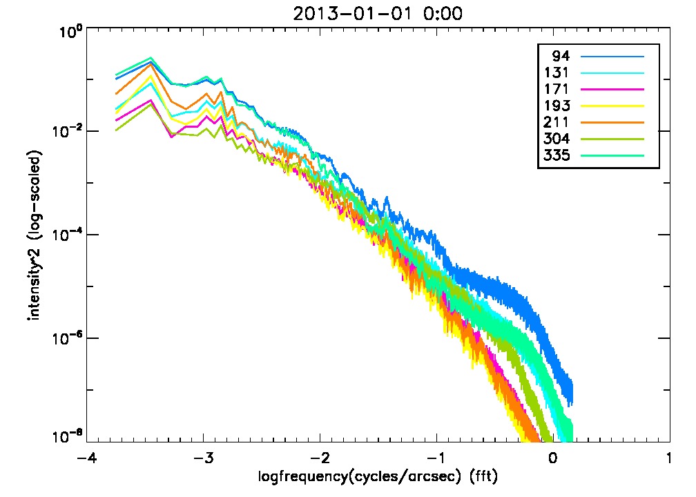
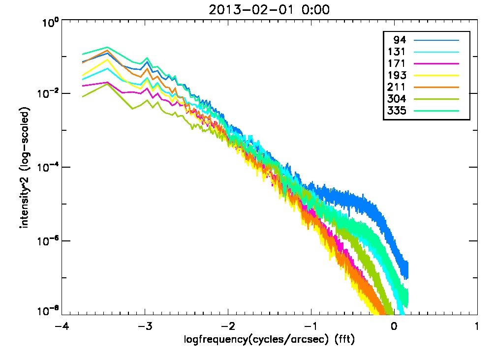
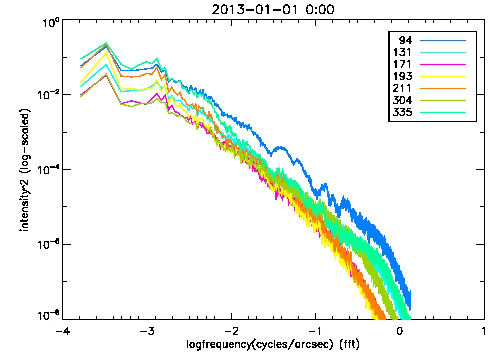
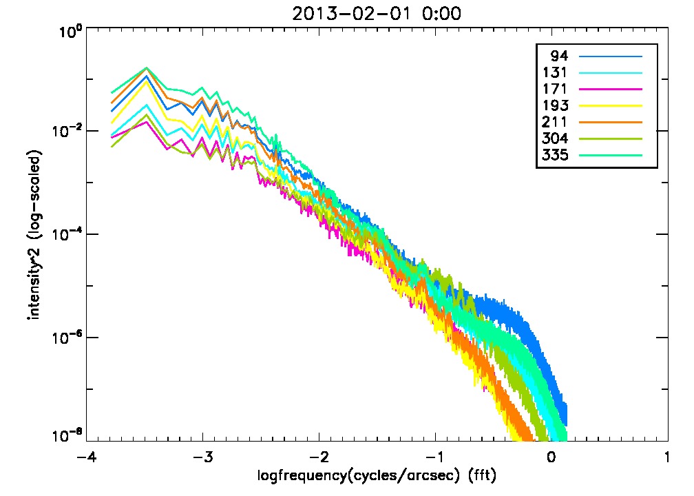
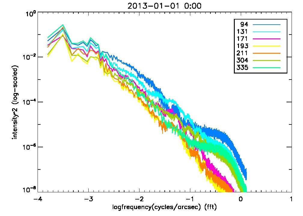
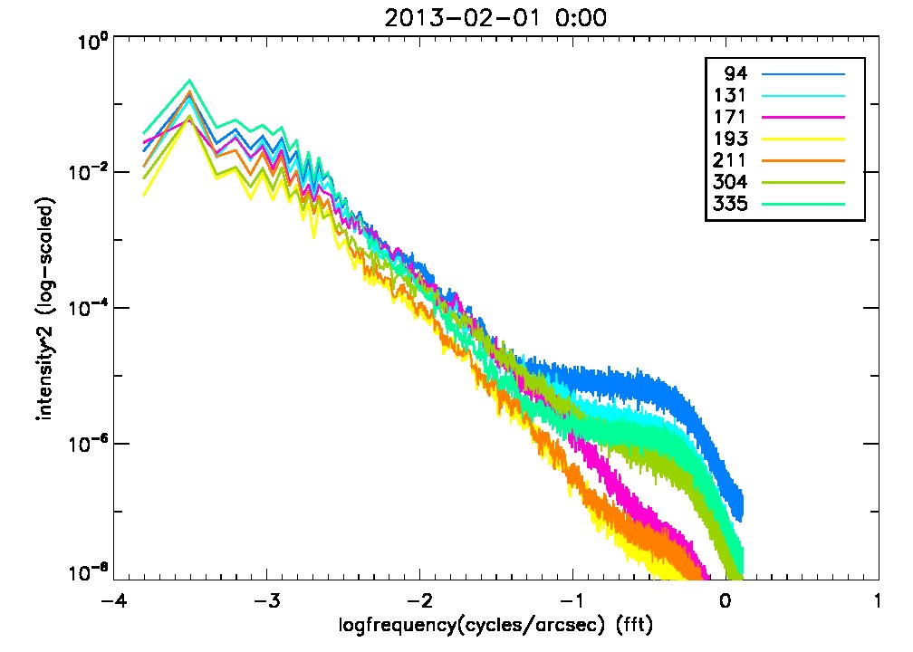
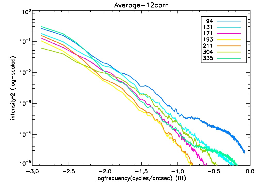
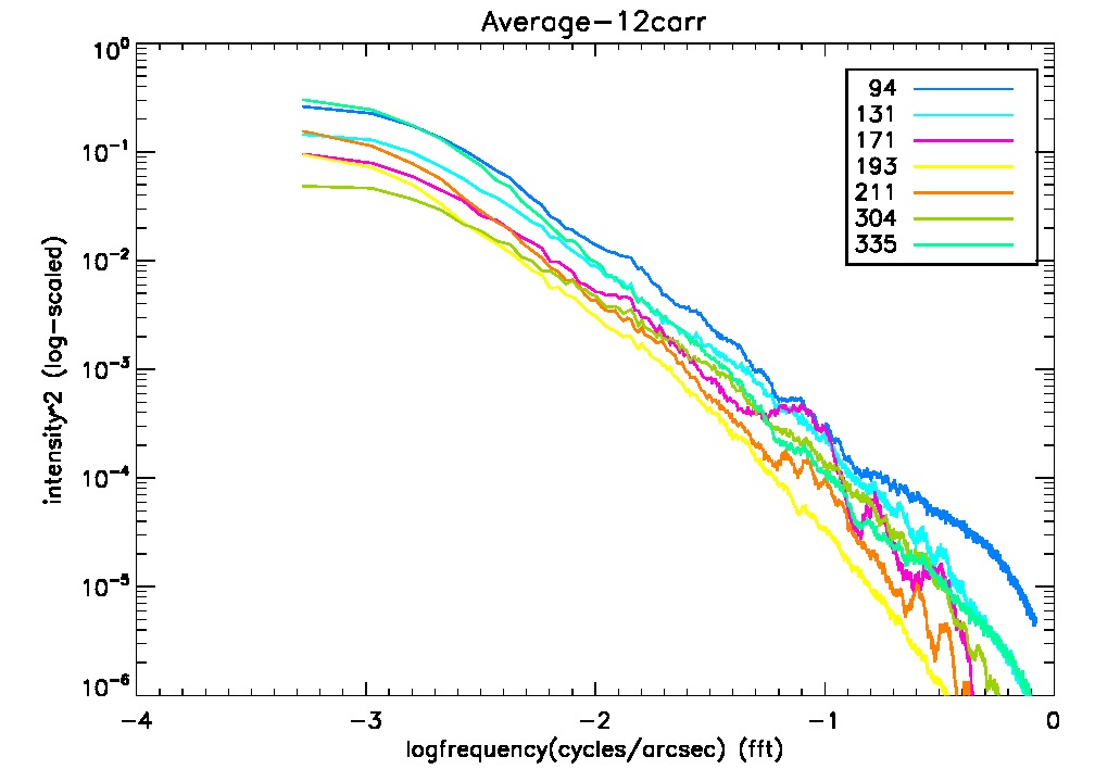
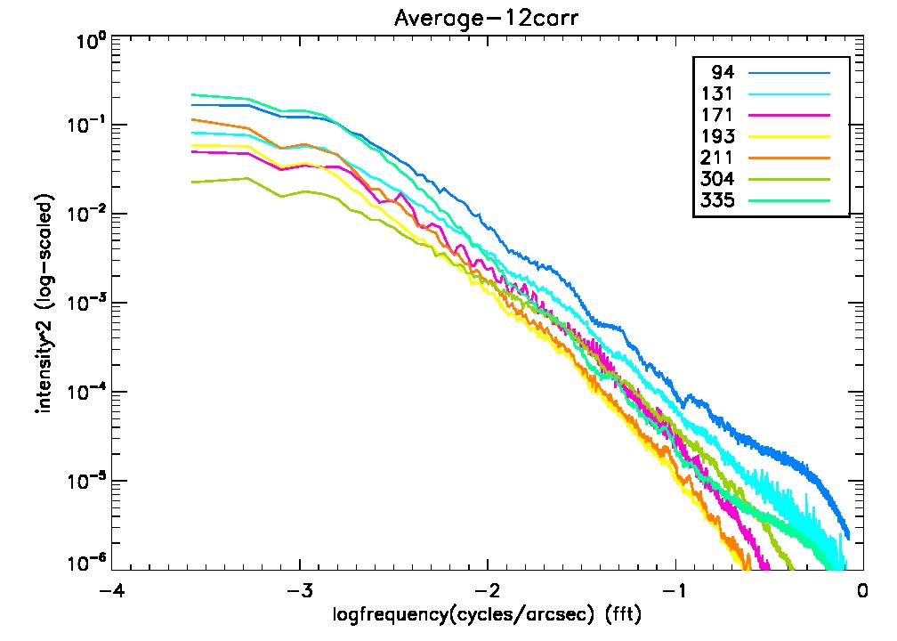
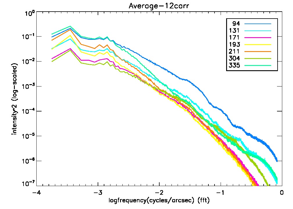
I finished running the "new" code. Now i have histogram, fft and contrast/75per/25per plots for 6 different sets of data corresponding to roughly a full Carrington rotation of the sun. The cadence used for the images was 86400 seconds (24 hours). Below are the fft plots for the first two sets.
200-205


500-505


1000-1005


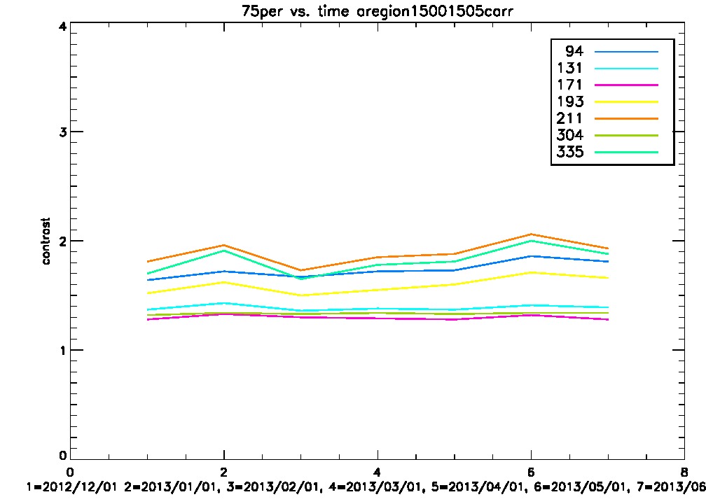
1500-1505


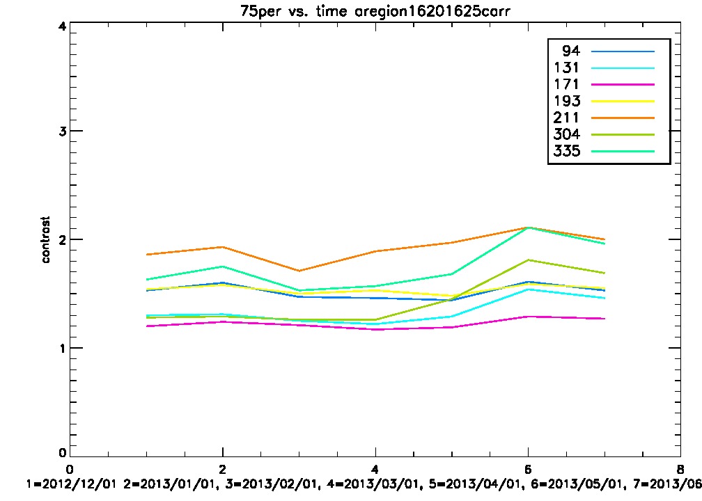
1620-1625


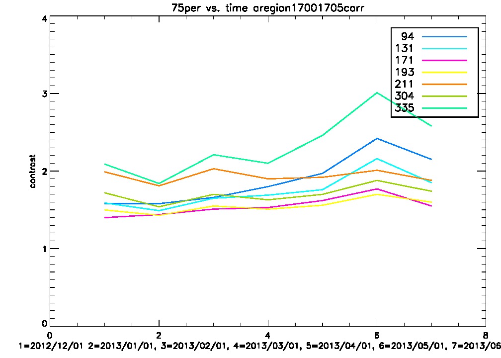
1700-1705


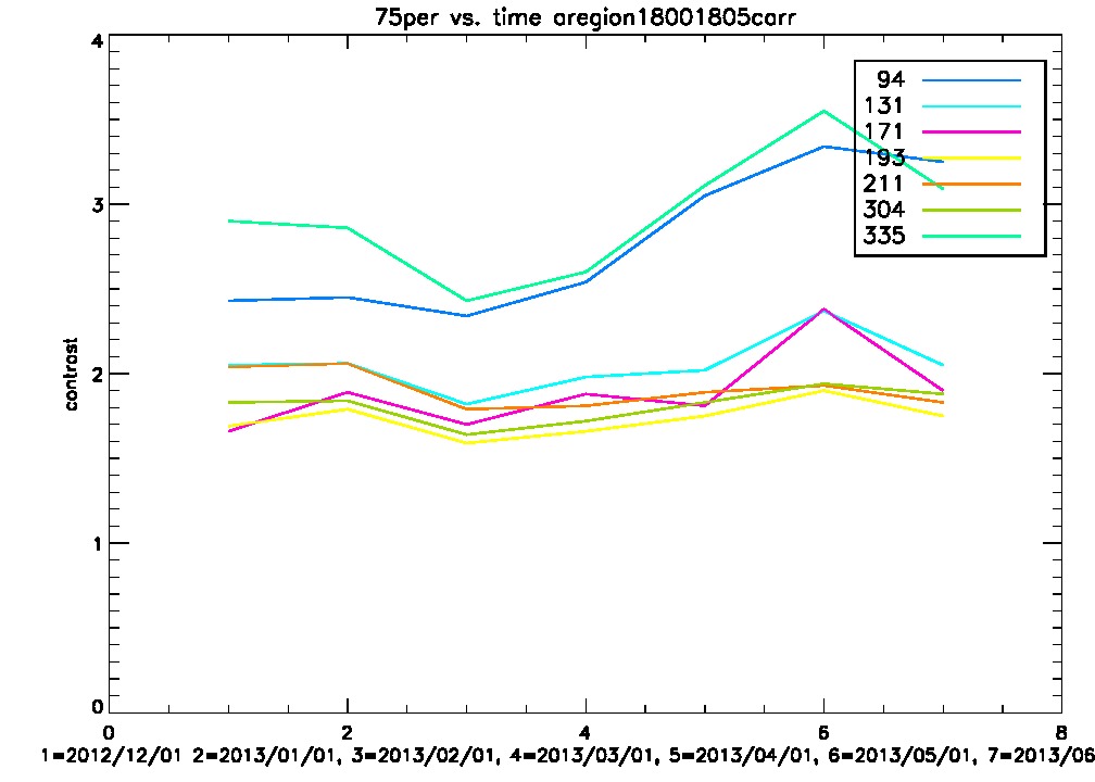
1800-1805


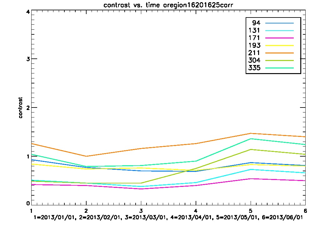
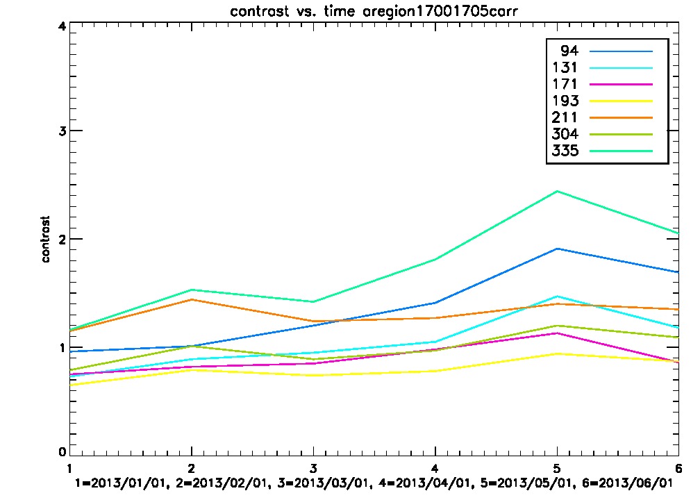
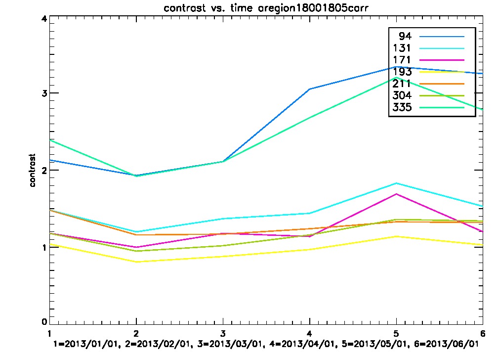
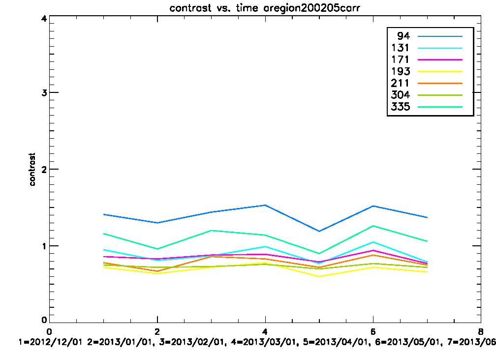
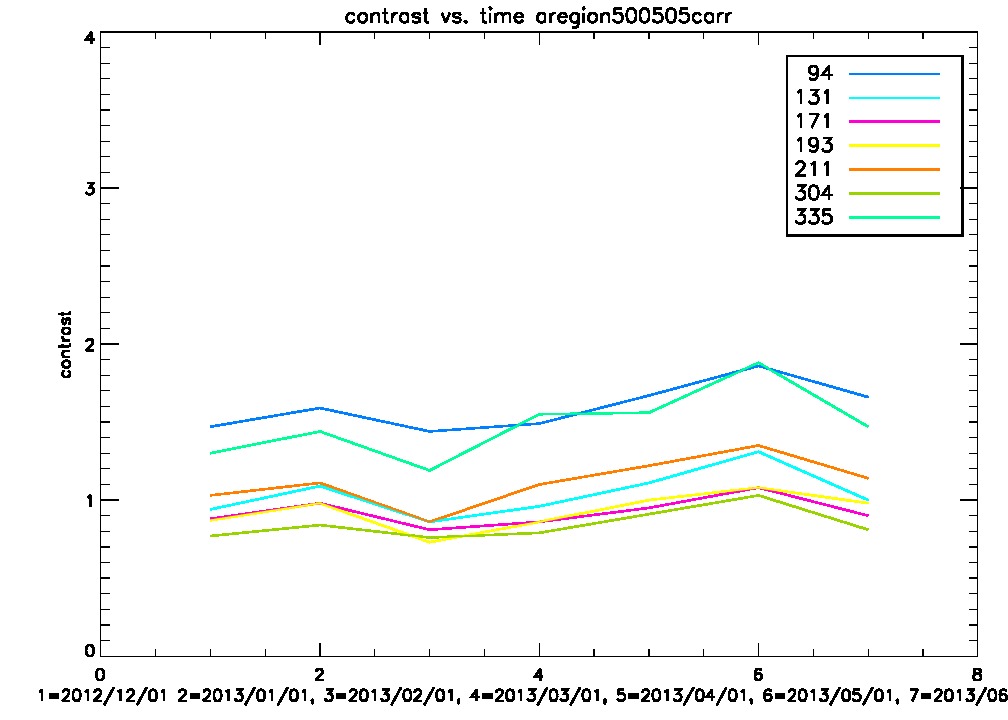
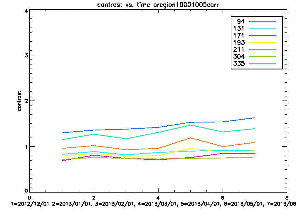
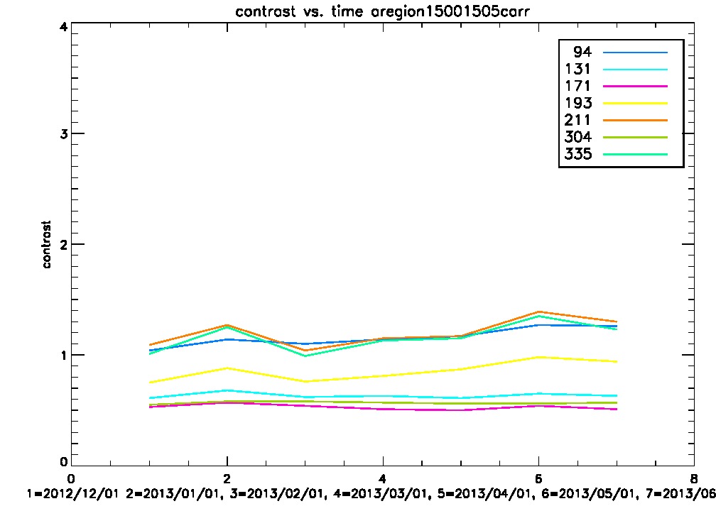
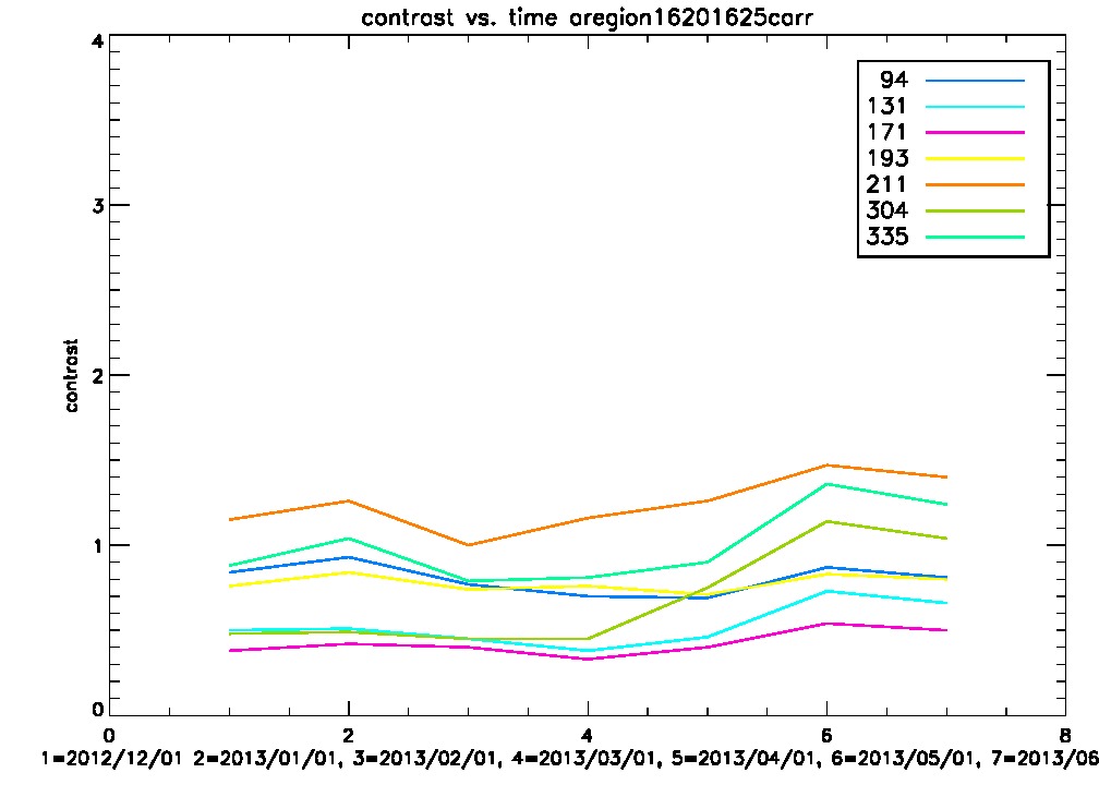
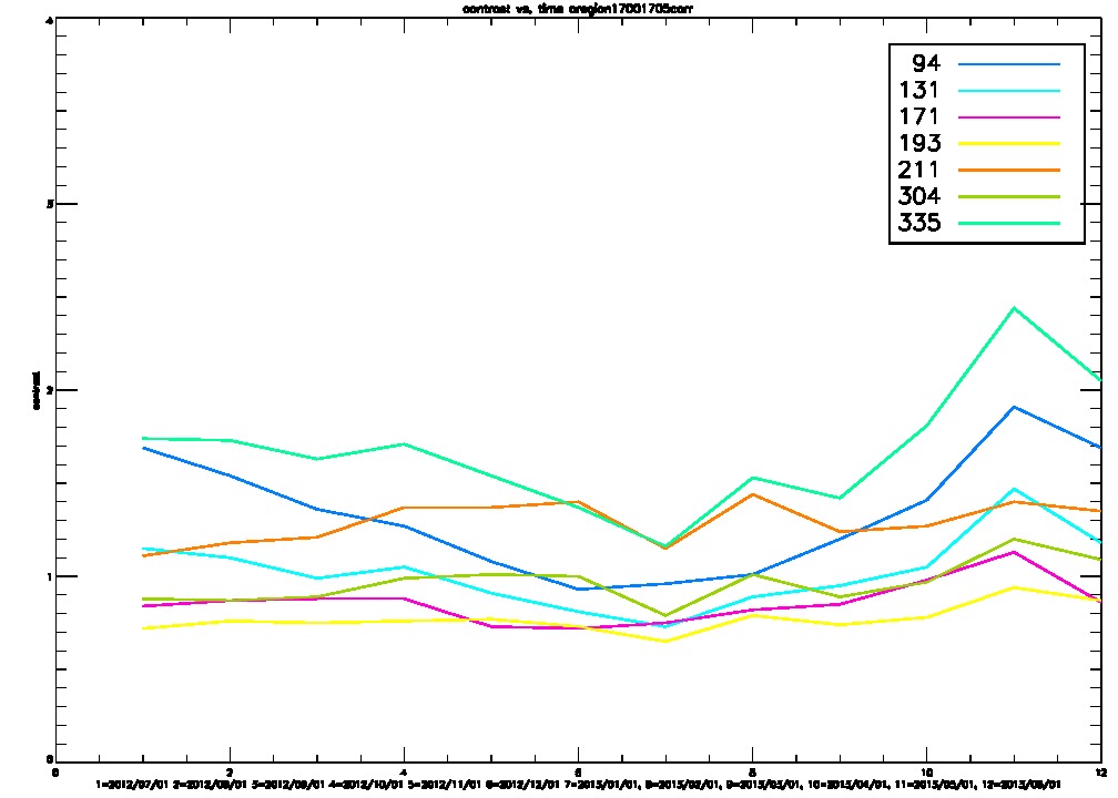
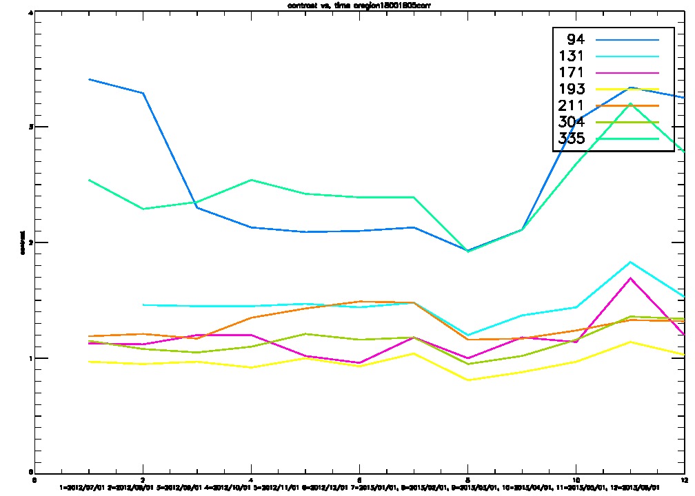
Contrast


07/19/2013
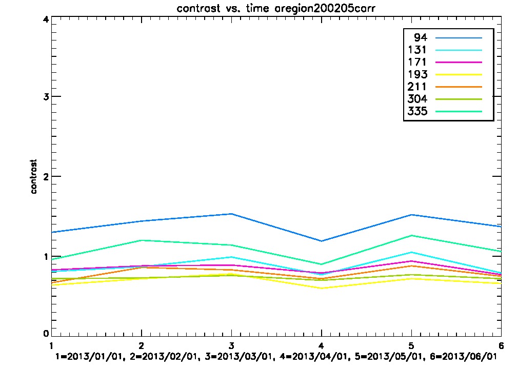
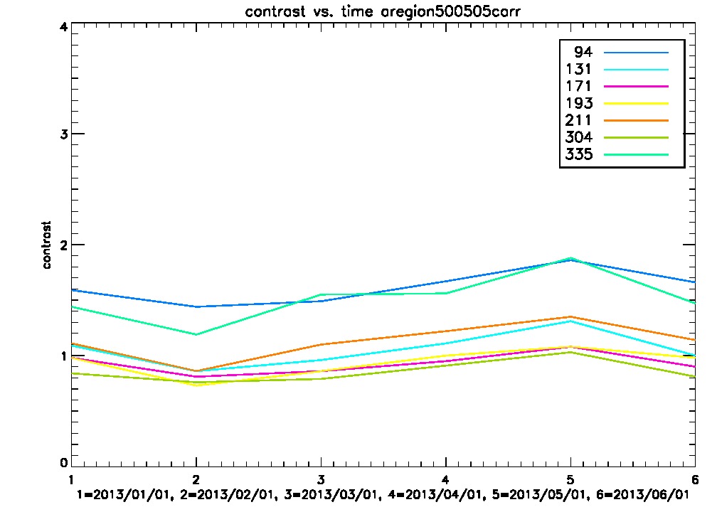
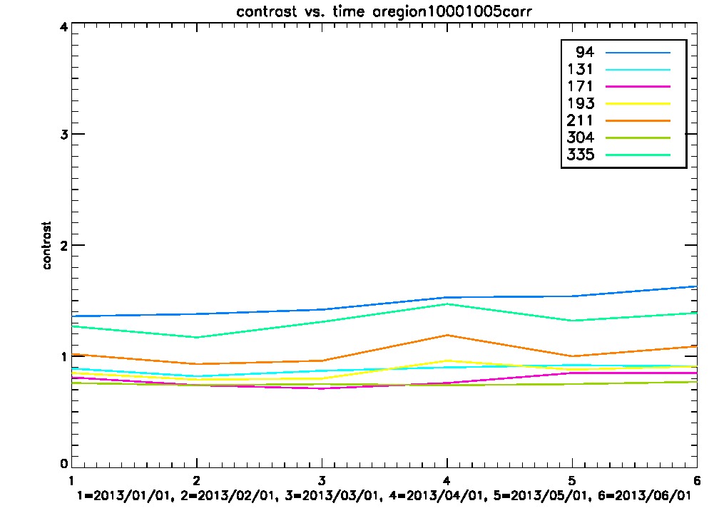
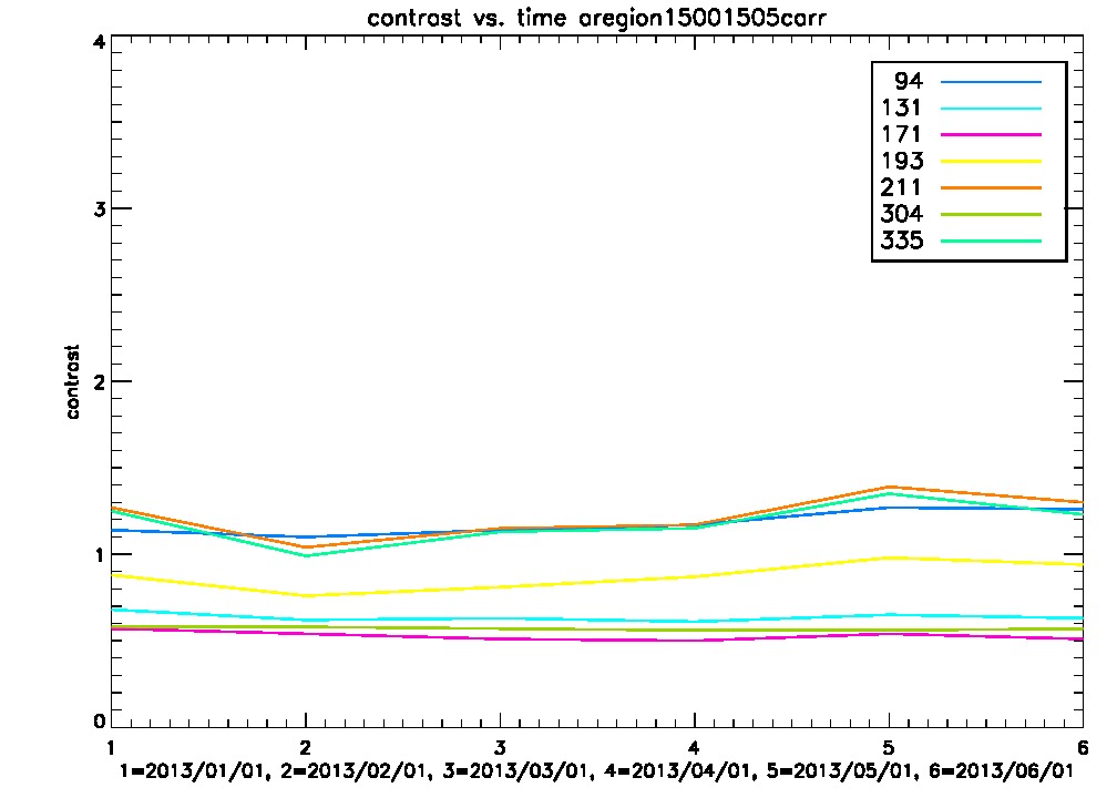
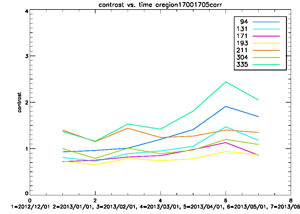
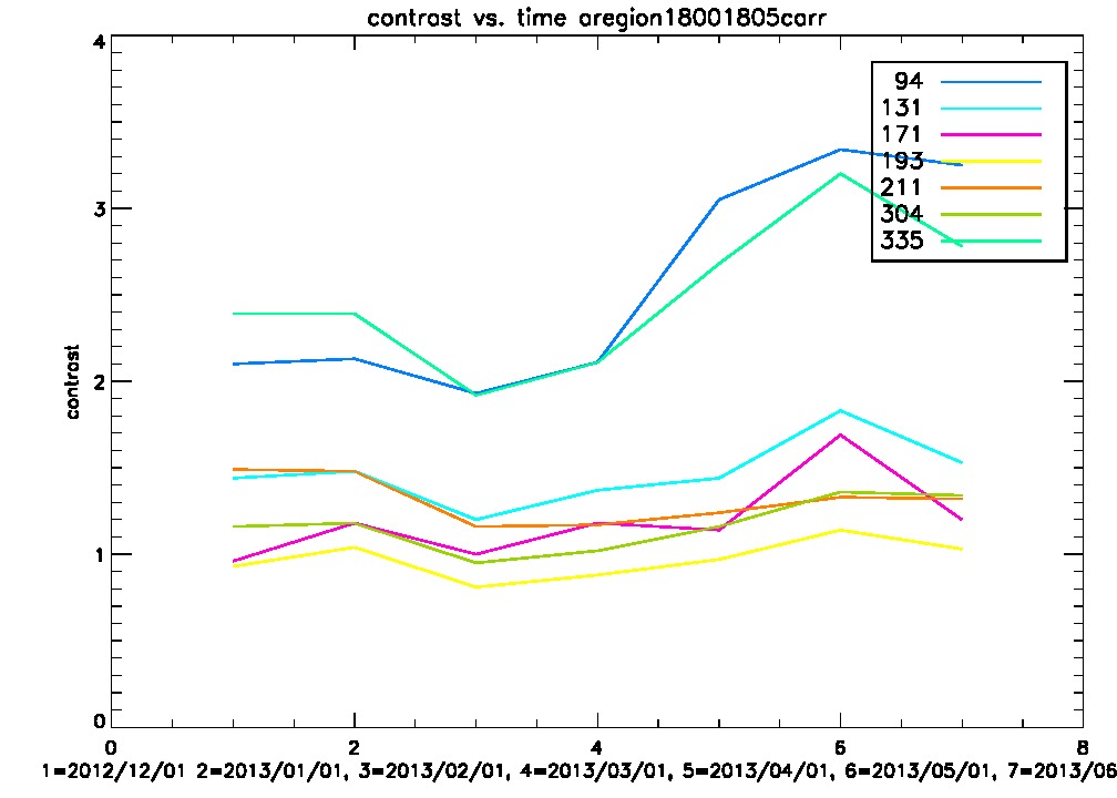
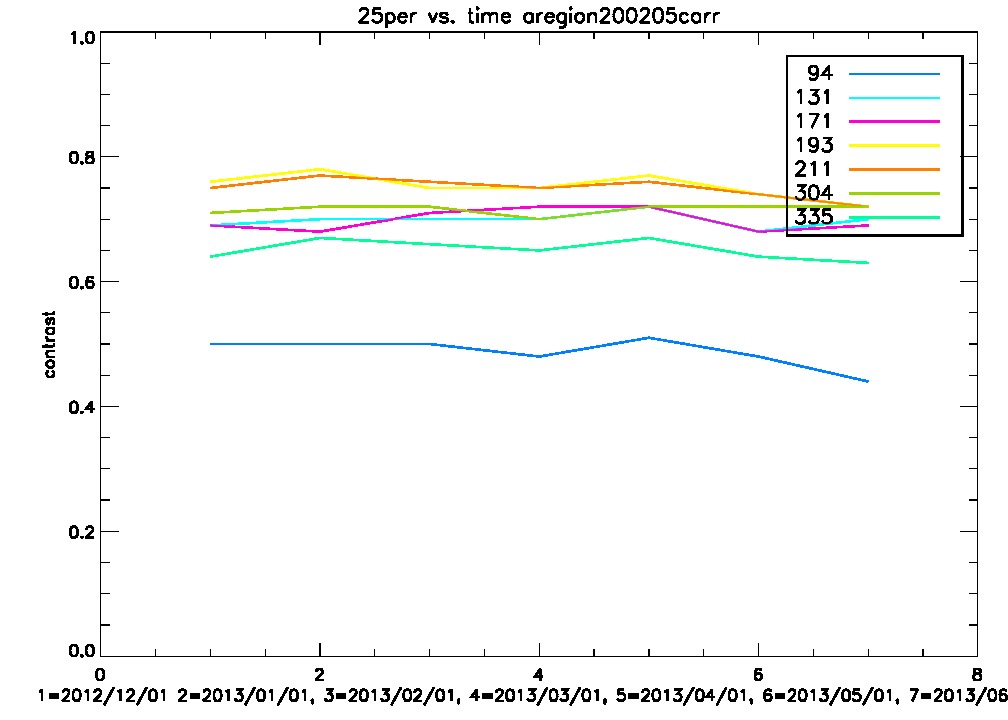
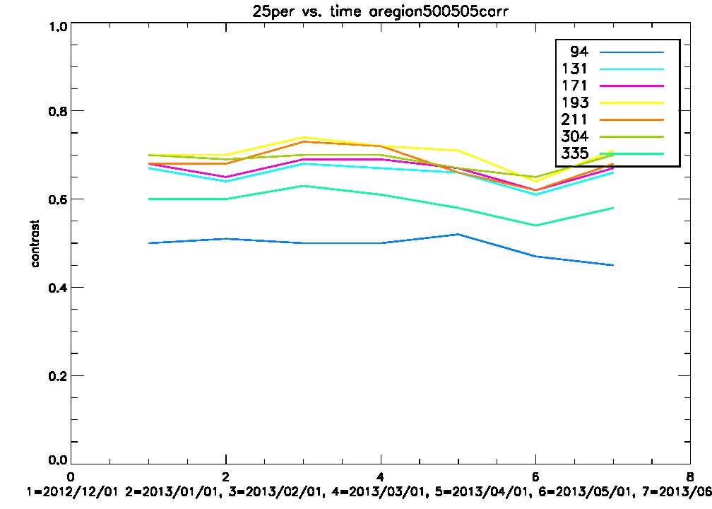
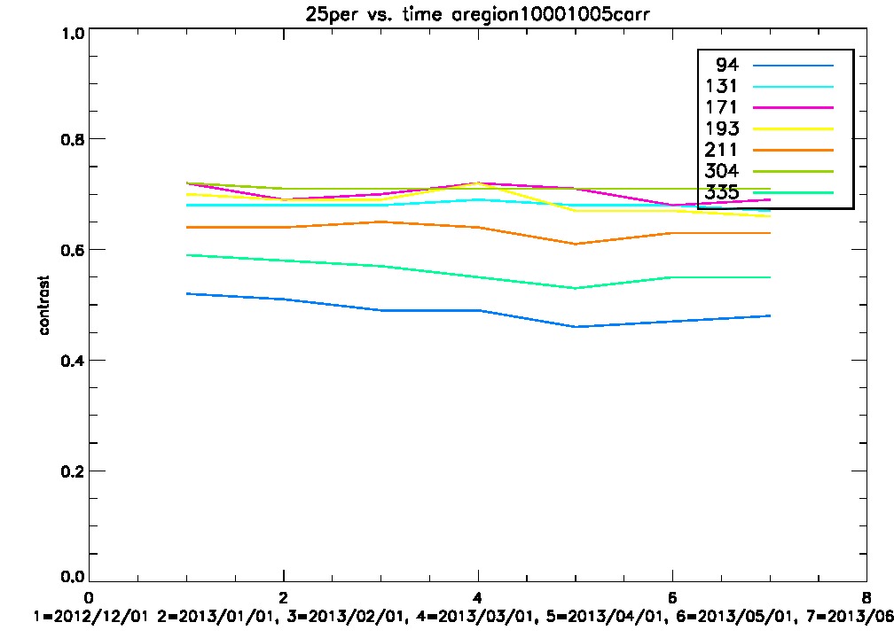
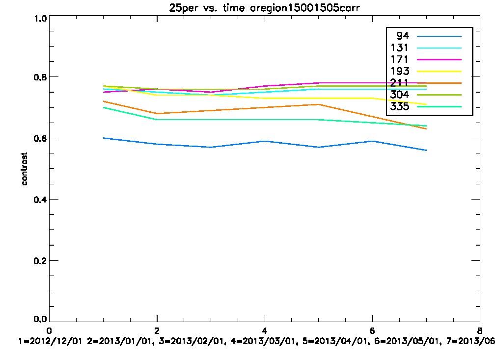
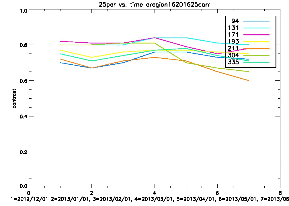
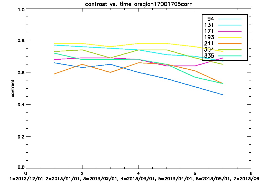
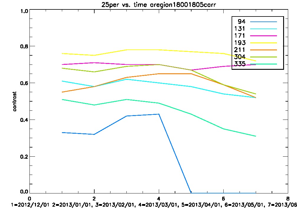
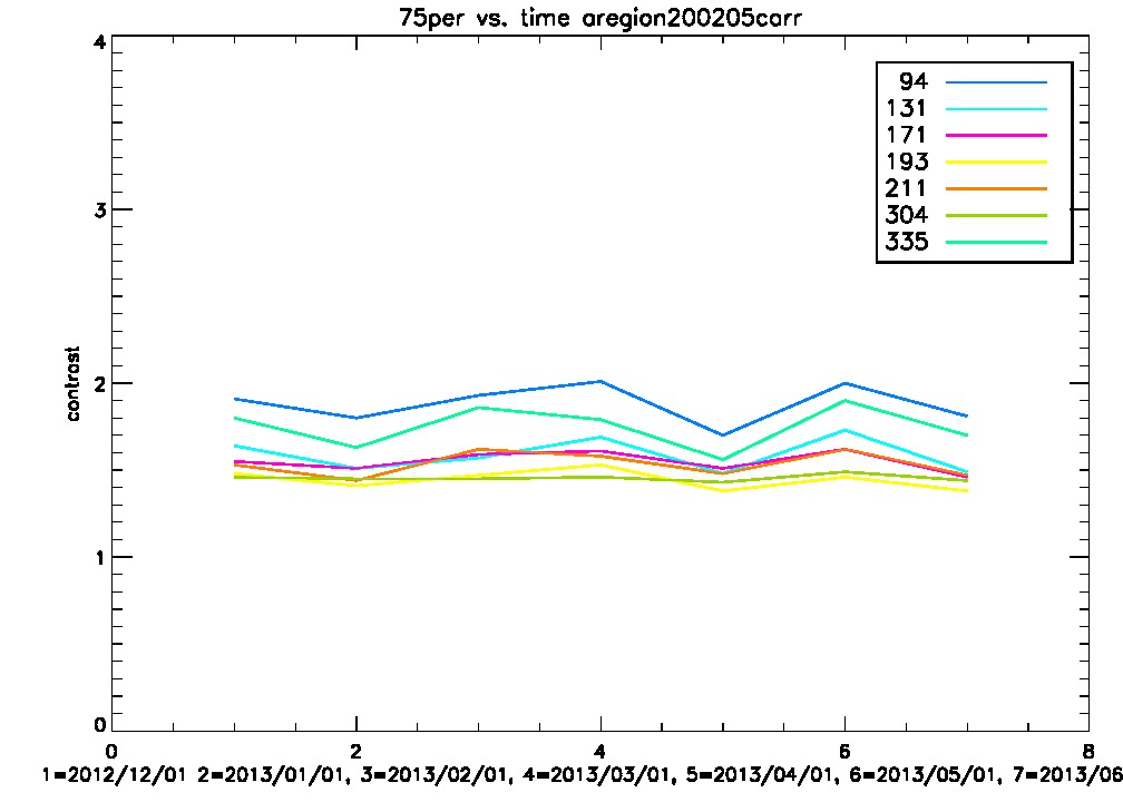
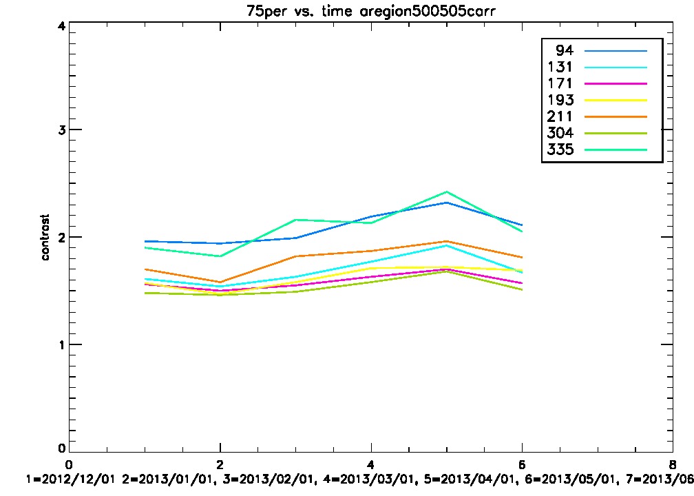
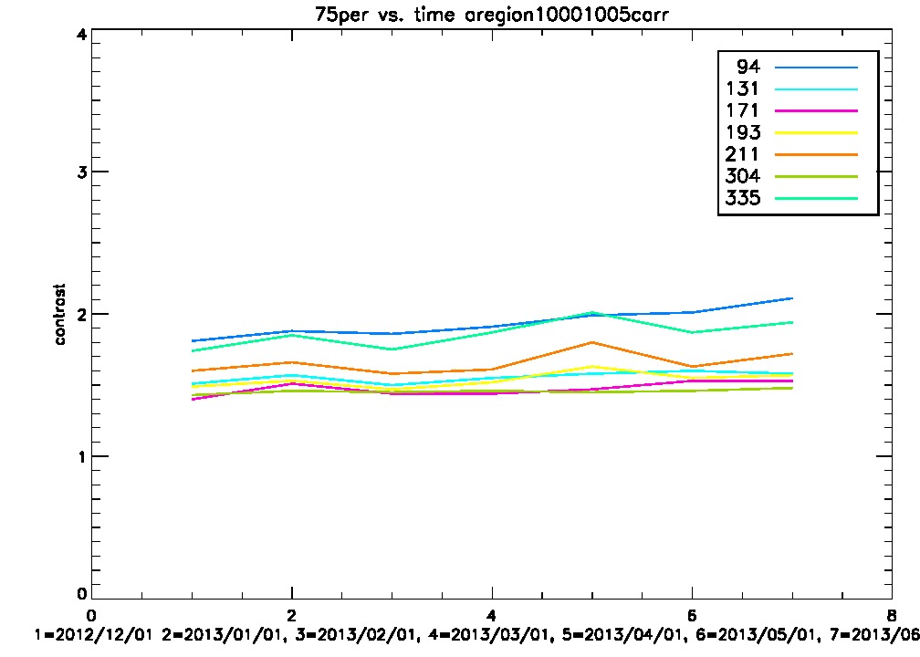
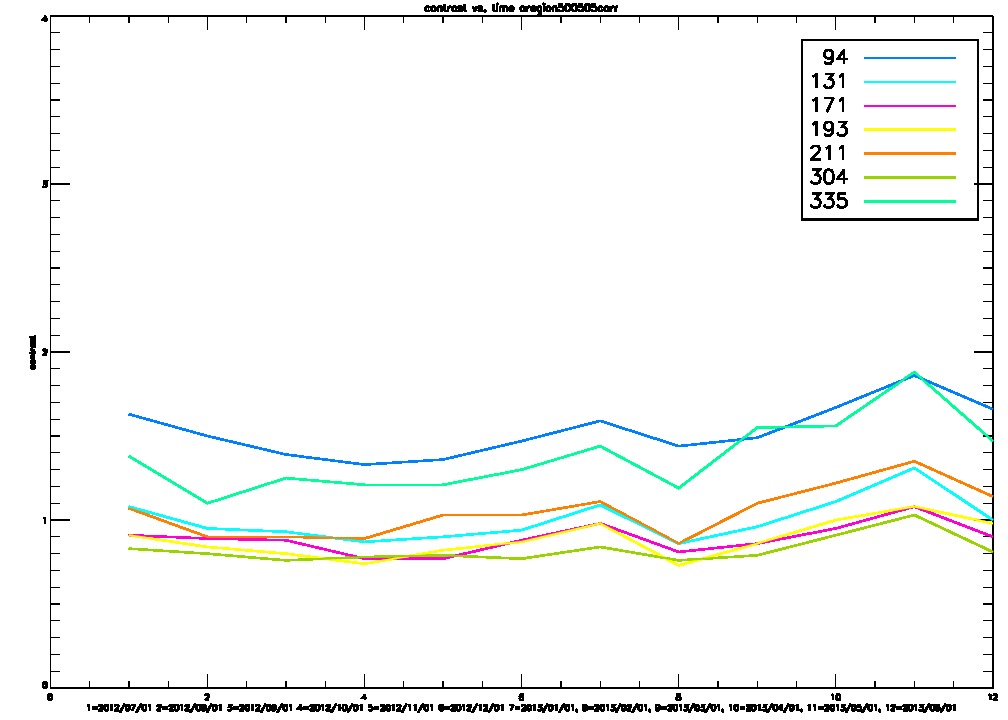
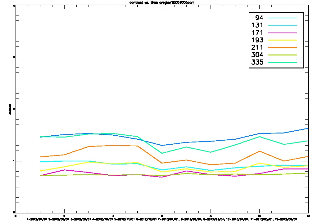
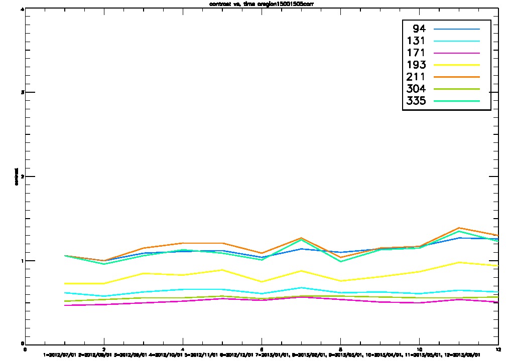
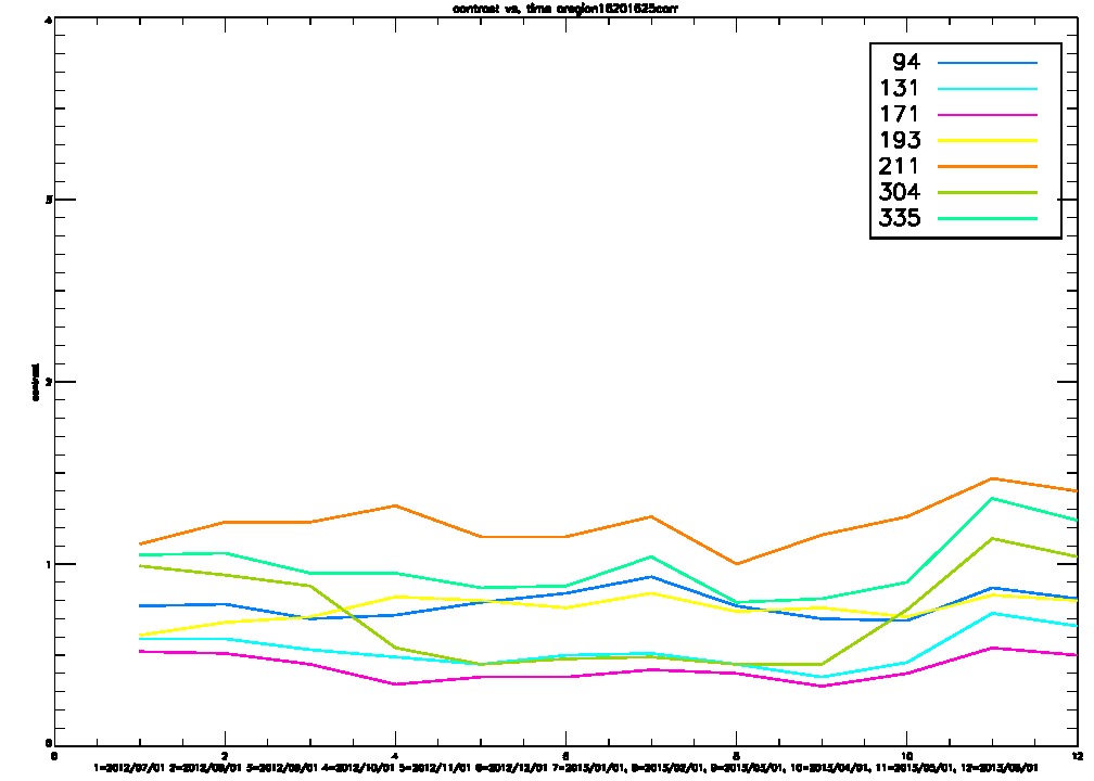
Contrast/25/75 plots for 7 sets of images.
Contrast


25th percentile


75th percentile


7/22/2013
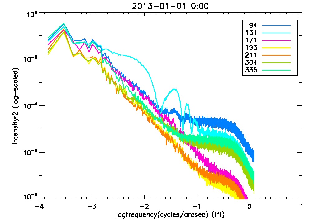
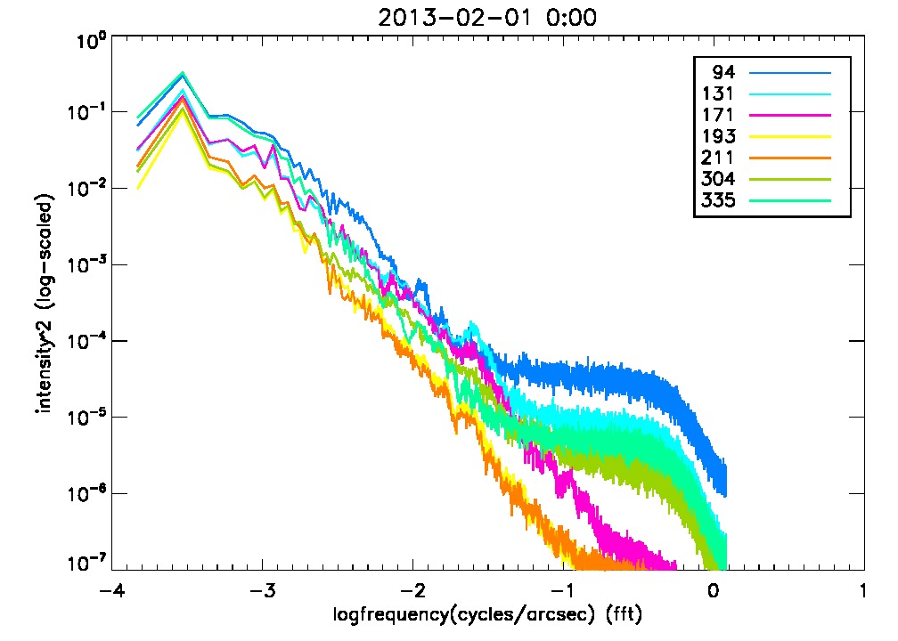
We can observe that the fft plots present two bumps. The location of these bumps varies between the different wavebands but is consistent troughout the different sets of images.It is also evident that the 335 and 94 angstroms wavebands present the highest contrast while the 304, 183 and 171 present the lowest contrast. We obtain similar results from each set we analyze but the most consistent wavebands seem to be 171 and 304.
7/25/2013
We have been trying to find an explanation for the bumps on the fourier transform plots. We have also been adjusting the x-axis of the fft plots to go from 0 to the Nyquist frequency.
We have been looking for the corresponding lenght scales (and frequencies) of different solar structures to see if any ony of them can be held responsible for the bumps. These facts are presented below.
Sunspots: ~33 arcsecs
Granules: ~1.4-2.0 arcsecs
Supergranules: ~49 arcsecs
Coronal Holes: ~974-1252 arcsecs
Active Region Loops: ~14 arcsecs
Spicules: ~.7 arcsecs
8/8/2013
Below are the plots presented in my final presentation. The plots are averaged over 12 carrington rotations of the sun (roughly)
Fft plots


Histograms


Contrast


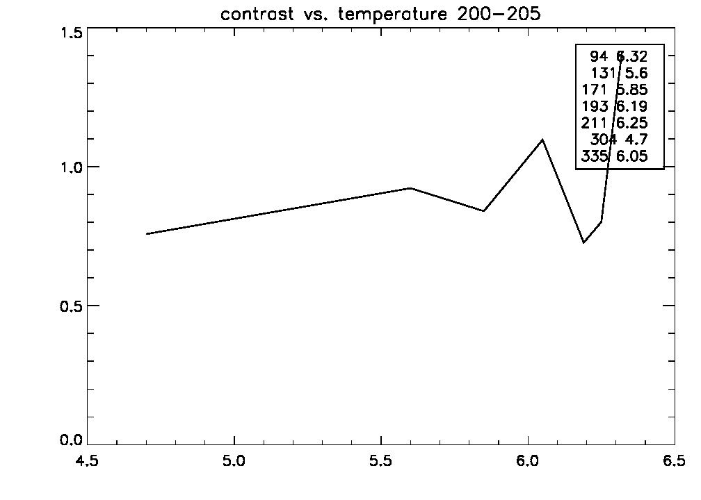
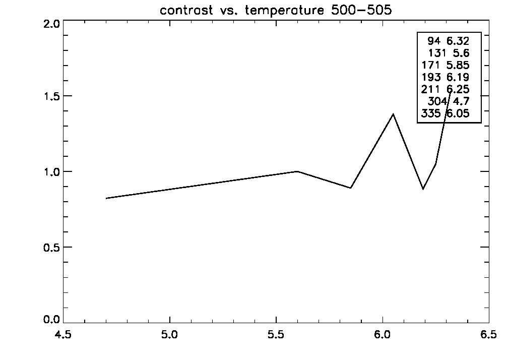
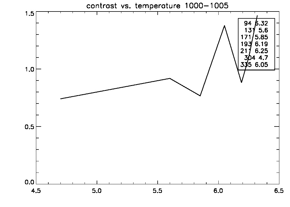
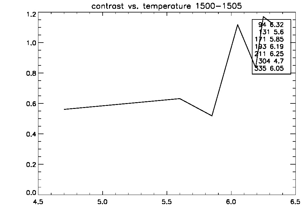
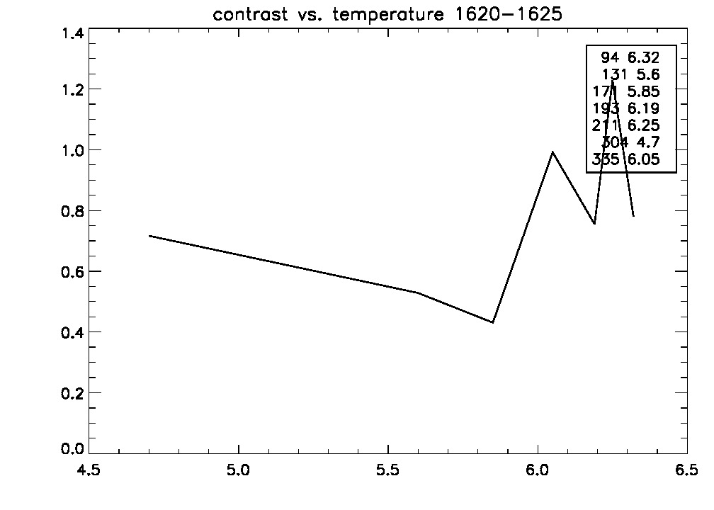
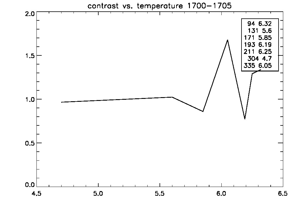
Contrast vs. Characteristic Temperature


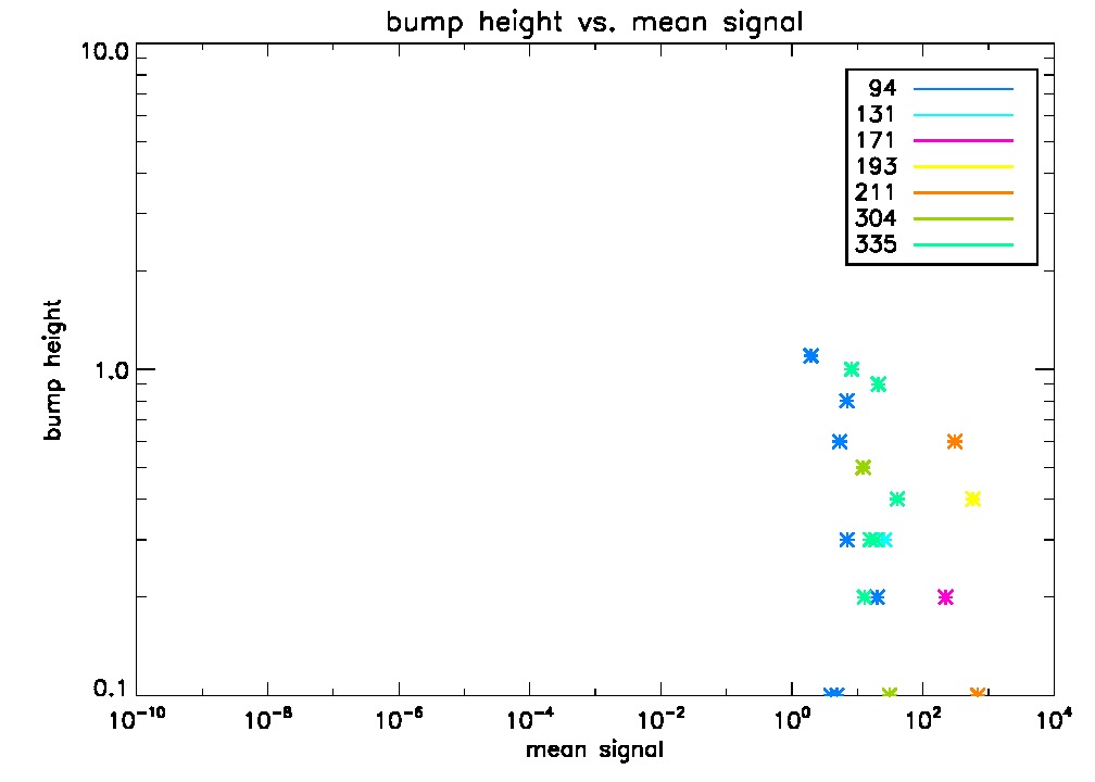
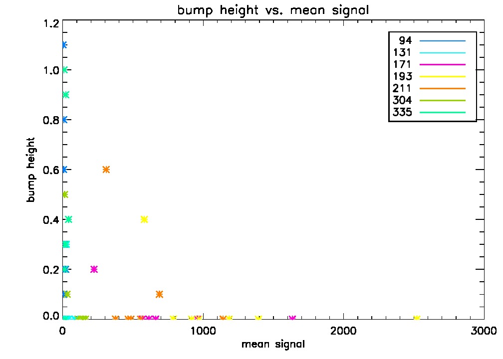
Bump Height vs. Mean Signal

Bump Height vs. Mean Signal (log-scaled)
