Week 10
I have finished data analysis to the best of my ability within the time constraints, and have coronal temperature analysis and volume emission measure (assuming isothermal plasmas) for 2008-2012 to show for the final project. The 2012 data is unreliable (this was when special processing (that I ran out of time for) of the data began due to increased light leaks, filter degredation, ccd buildup) and contains several errors, but the general trend of temperature is easy to see, and that is what I deemed most important.

My final project presentation can be found here.

Week 9
This week, I finished preparing the 2008-2012 data for temperature analysis. I will be analyzing the temperature of the full corona (extrapolated geometrically from energy and emissivity of the disc), as well as the northern hemisphere and southern hemisphere. This will be presented next week at our research presentations.

Below is a graph of the temperature for December 2008. I chose December 2008 as it is the beginning of solar cycle 24.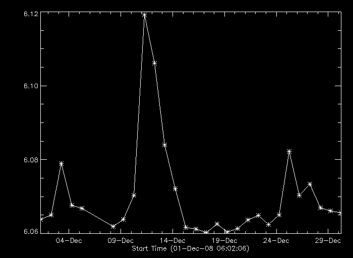

(y-axis in log-scaled MK, 10^6, roughly, in this case)

The volume emission measure (VEM) is plotted as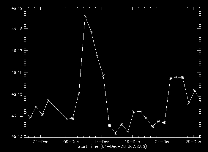

The VEM is given as the product number of electrons produced in the CCD squared by the volume of the plasma

Week 8
After last week's video malfunction, I spent this week looking at how to remedy the problem. I discovered that the arrays didn't have the same size, and discovered that it is because multiple images could match the time constraints (within 20 minutes) of one, so the other one was not being removed, leaving extras. I attempted to fix this, and the video for 2010 can be seen here, while the video for 2009 can be seen here.

The filter ratio method uses the ratio of the ccd counts of two images, using two different filters and taken at nearly the same time to deduce temperature. The ccd electron energy is calculated, assuming the corona is an isothermal plasma.

E is the energy of photons on the ccd measured using the energy of electrons on the ccd.

When the intensity is normalized and the ratio taken, the resulting equation is only a function of temperatue. The filter ratio method can be used for emission intensity as well.


F is defined as the XRT temperature response, which is different for each filter.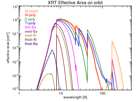




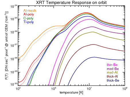
The results of the filter ratio can then be used to find the data number, which is a function of temperature. On the Hinode XRT, 1DN is 57 electrons.

(Graphs from Narukage et al., equations from Hara et al.)

Week 7
My task now is to begin selecting good images and data gathered at the same time for the titanium poly and aluminum mesh filters for the year 2010 for comparison and coronal temperature analysis. This must be done manually at this time. This technique will then be expanded upon for the full 11 year solar cycle / Hinode XRT activity. Perhaps there's an easier way using an algorithm to do this?

It was difficult to select which data to remove. It was my goal to have only pure data, that is data with no glitches or composite exposure problems, but it was decided to retain these datasets, as long as they don't cause a major irradiance dip, because having a large amount of data to compare between the two filters is important. The images must be taken around the exact time in both filters to be comparable for temperature analysis.

A movie showing both the al_mesh and ti_poly filter data for 2010, time matched for temperature analysis, can be viewed here.

Week 6
This week, I'm preparing for mid-research presentations, which mine can be viewed here.

Week 5
This week, I derived the irradiance of the northern and southern hemispheres of the solar disc for the full year 2010 with the aluminum mesh filter.

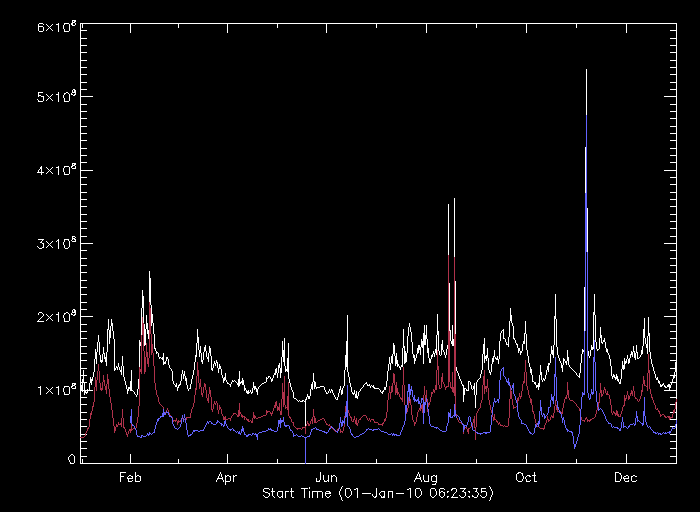
In this graph, the northern hemisphere appears red, the southern blue, and the full disc white. This graph is incorrect as some data is still missing for the southern hemisphere in January; however, this can be fixed and the basic principles implemented for a full year movie showing the northern and southern hemispheres alongside the full disc for the project mid-term presentations next week.
I noticed that, for the year 2010, the most active regions appeared in the northern hemisphere, aside from the very active region that peaks in early November in the south.

Last week, Allison helped me develop a program that selected the first and last images taken each day to create a smoother movie. By helped me, I mean that she did all of the coding, while I was only able to help with the pseudo-code, as some of the IDL was beyond my expertise. The only flaw in this code is that it does not account for bad data, and it is not useful to study the full irradiance, as some active regions may change drastically throughout one full day, and that data may be missed in this movie. This new movie also normalized all frames around the same overall log scale, instead of scaling them individually, which allows for more consistent intensity of the images. That movie can be viewed here. A six month version of this movie for the second half of the year showing the pattern in irradiance that we discussed will be finished either tomorrow or next week.

Week 4
This week, I was exploring the point about the irradiance spike in November 2010, as well as the cyclical nature of the irradiance over a one month period. Below is a graph of the irradiance of the corona with the titanium poly filter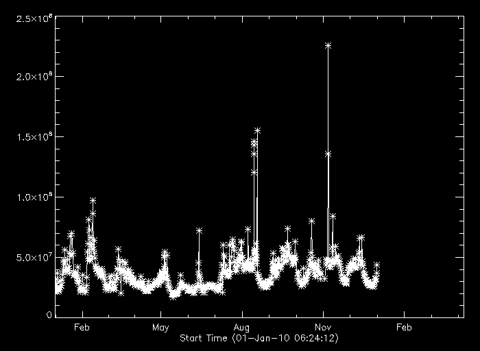

The spike around early November is evident with this filter, as well as the aluminum mesh filter. This lowers the chance of it being caused by an over-exposed composite image.
I discovered that the spike is caused by an active region, which created a spike in irradiance that lasted for only one day, November 6th. The active region that causes this spike in November can be viewed in a movie here. I also noticed that there is a much greater ccd count for the aluminum mesh filter than the titanium poly filter.
The full year movie for 2010 of the x-ray spectrum on the solar disc using the aluminum mesh filter is available here.

Week 3
This week brought a challenge of creating a program that would assemble all structure data from each dataset for the year of 2010 into one to be plotted with the irradiance data itself. This proved to be more difficult than expected; I'm still struggling my way through IDL, but my understanding is definitely improving this week.
I also was tasked to produce the same year graph for the titanium-poly filter and comparing it with the aluminum-mesh filter. Below is an image of the irradiance for 2010 with the aluminum-mesh filter. Along with this, I was asked to think of a way to script a program that would analyze the solar irradiance for only the northern or southern hemisphere of the solar disc.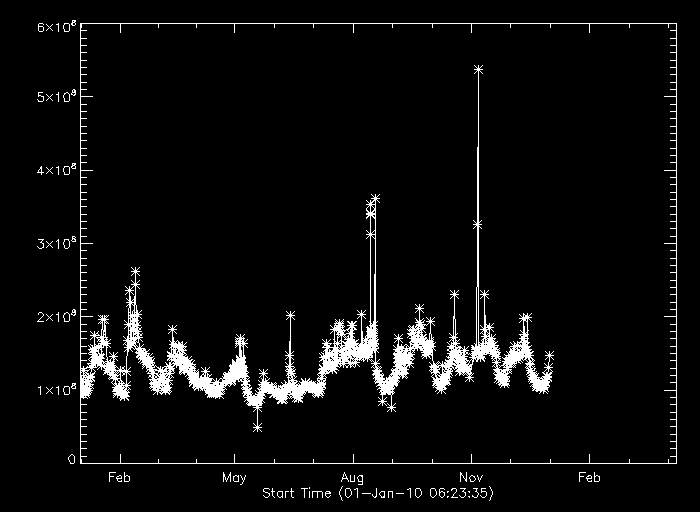

Week 2
I spent the week struggling with IDL to collect graphical data of the irradiance, that is, the x-ray photons incident on the ccd.

Week 1
I spent the week getting familiar with the Hinode mission, with Keiji's help, while Aki was out of town.