Investigating solar Lx-B relation: with Hinode/XRT and SDO/HMI.
Nathaniel Cohen (California State Univ.) with Aki Takeda
as a MSU solar/space REU 2026 project.
Project description
Our Sun is a G type star with the surface temperature at around 6000(K),
but its thin atmosphere called corona is known to be more than 300 times
hotter than the surface. The heating mechanism of the corona above the
cooler surface is not fully understood, but the magnetic flux penetrating
the surface from Sun's interior is believed to play a crucial role.
This project explores the possible heating mechanism by closely comparing
the coronal X-ray luminocity (Lx: measured as soft X-ray intensity) with
the photospheric line-of-sight magnetic field (B: obtained from spectral
information of visible light).
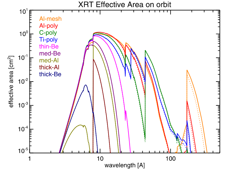
We will use data acquired in space. As soft X-ray data, we will use X-Ray
Telescope(XRT) aboard the Hinode satellite (an international mission among
Japan/US/UK), As magnetic field data we will use Helioseismic and Magnetic
Imager(HMI) aboard the Solar Dynamic Observatory (a NASA mission). Student
will first learn about these instruments and basic calibration of the data.
The data analysis will be performed using IDL (Interactive Data Language)
software. Experience with IDL programming would be favorable, but not
required, as the basic programs will be provided.
This REU project started in 2024 as an extension of the study described
in Yoshimura et al (2025) , which uses the full-Sun integrated signals
of soft X-ray and magnetic field images. In the past two years, Lx-B
relation for the sunspots was investiaged. This year, this project will
further expand the object of research to other solar structures like
coronal bright points and quiet Sun.
 |
 |
Weekly goals
- Week 1 (5/26 -- 5/29) :
- attend Python and IDL tutorials.
- background study (flare class, GOES, solar coordinates, etc.)
- lend out "Encyclopedia of the Sun".
- Week 2 (6/1 -- 6/5) :
- Study of the instruments: Hinode/XRT and SDO/HMI.
- Preparation for the short presentation on Friday 2pm.
- Week 3 (6/8 -- 6/12) :
- Data selection (select dates from SCIA).
- Understand image co-alignment (XRT & HMI).
- Pick up XRT bright points and corresponding HMI structures.
- How to prepare personal web site (uploading the presentation file).
- Week 4 (6/15 -- 6/19) :
- XRT intensity readings of selected bright points
with two filters (Al_mesh and Al_poly).
- Preparation for the group meeting on Friday 2pm.
- Week 5 (6/22 -- 6/26) :
- Nathaniel's last year's REU experience at Prinston Center for Complex Materials.
- Conversion of intensity to Te and EM.
- Preparation of AAS/SPD meeting attendance (8/10-14 in MD).
- create an account on the SPD meeting site
- searching for available flights to/from MD
- Week 6 (6/29 -- 7/3) :
- Preparation of mid-term presentaion: supporting plots of filter ratio method
[memo: created by xrt_resp/get_fratio_amap_ch1102.pro]
- Mid-term comment: Histogram study for BPs would be useful (by Dana).
- Week 7 (7/6 -- 7/10) :
- SPD abstract submitted (7/6).
- Add more data from the period around solar minimum.
- 2017/12/29 (by Nathaniel)
- 2020/02/12 (by Nathaniel)
- 2021/01/08 (by Nathaniel)
- 2018/07/09 (by Aki)
- 2019/05/19 (by Aki)
- 2020/05/13 (by Aki)
- Week 8 (7/13 -- 7/17) :
- To get more data points for a wider range of QS,
apply larger or smaller FOV size to solar minimum data.
- Try linear fitting of BP and QS data points (poly_fit)
- Make histogram for Te, EM and Luminocity.
- Plot with error bars.
- Prepare for the group meeting presentation.
- Week 9 (7/20 -- 7/24) :
- Add more minimum data (2020/02/12, 2021/01/08) with smaller FOV.
- Replace full-Sun data with the Chianti 11.02 version.
- Try other B_cutoff valued: 0G, 45G etc.
- Make histogram for Te, EM and Luminocity with solr min subset.
- Estimate uncertanty in a reasonable way.
- Set goal (conclusion) of our study.
- Week 10 (7/27 -- 7/31) :
- Create poster for REU(7/29) and SPD(8/10-14).
- Prepare for the final presentation on 7/30.
Resources
|