June 15, 2009
Today’s
lecture was given by
Dr. Dick Canefield,
his
lecture focused on
radiation in space. One of the
only
ways scientists are able
to study astrophysics is
through
radiation. He
discussed continuous radiation,
line
radiation, thermal/ non-
thermal radiation,
emission/
absorptions, and
photon mean free path.
After
the lecture I met up
with Angela and she was able to help me
resolve some of my problems with my program but there seems to be a
problem with Dana’s programs that will allow me to rotate the topology
to match the RHESSI data. A quick fix was to rotate the RHESSI data to
match the topology but a minor problem occurred, the topology was not
fitted to the magnetogram properly.
I
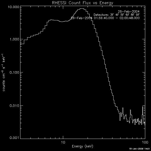
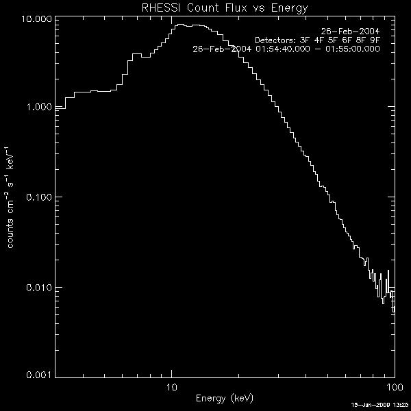
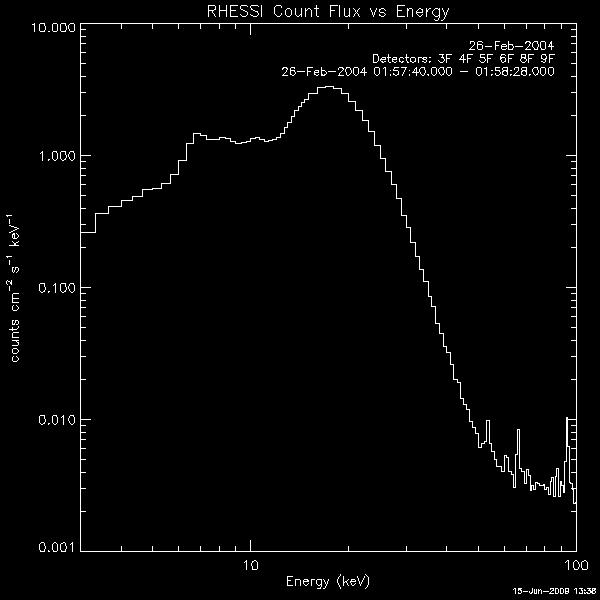
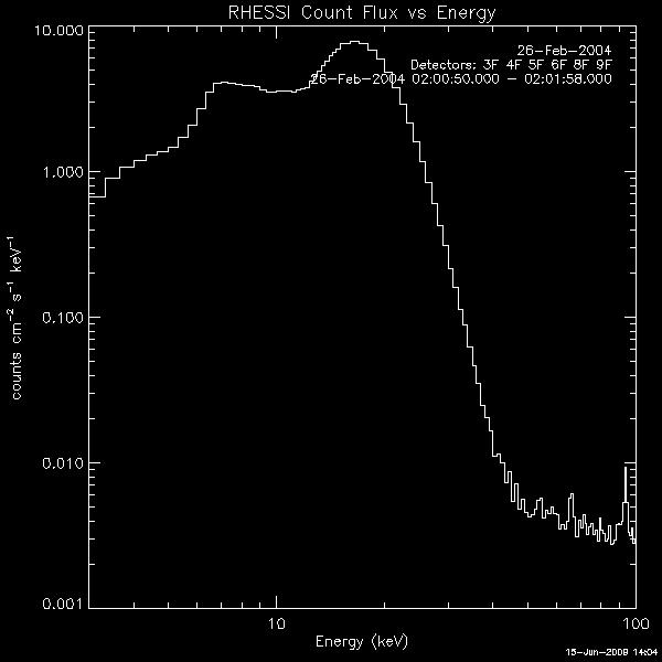
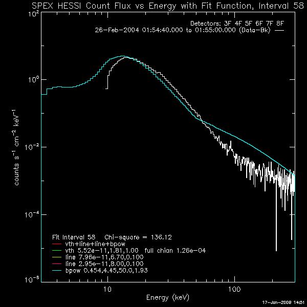
started to break down the
spectrum into smaller intervals.
Time
start-1:54:40
Time
end- 1:55

Time
start-1:57:40
Time
end- 1:58:30

Time start- 1:58:30
Time
end- 1:59:40
Time
start-1:59:40
Time end- 2:00:50

Time
start- 2:00:50
Time
end- 2:02:00

Time
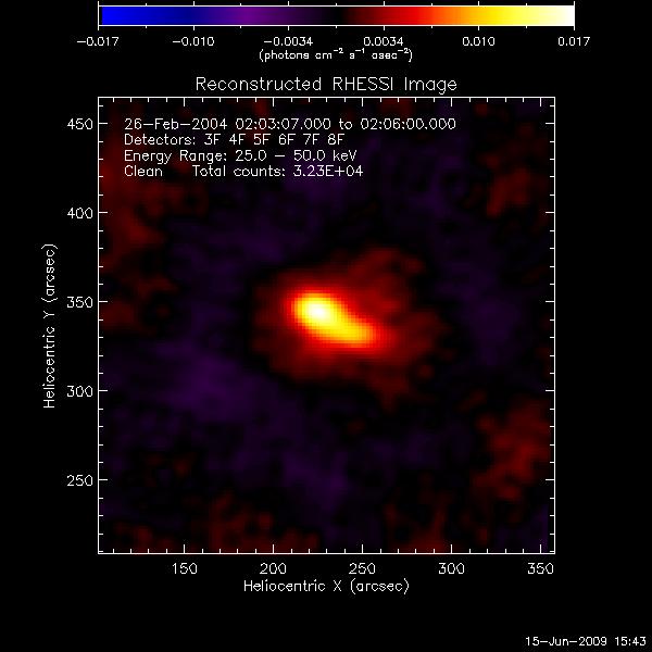
start- 2:03
Time
end- 2:06

I
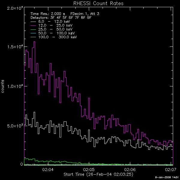
then created a light curve for the time period 2:03:07 to 2:06
which allowed me to see if I had an accurate amount of counts to make a
RHESSI image.

I
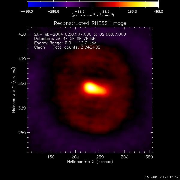
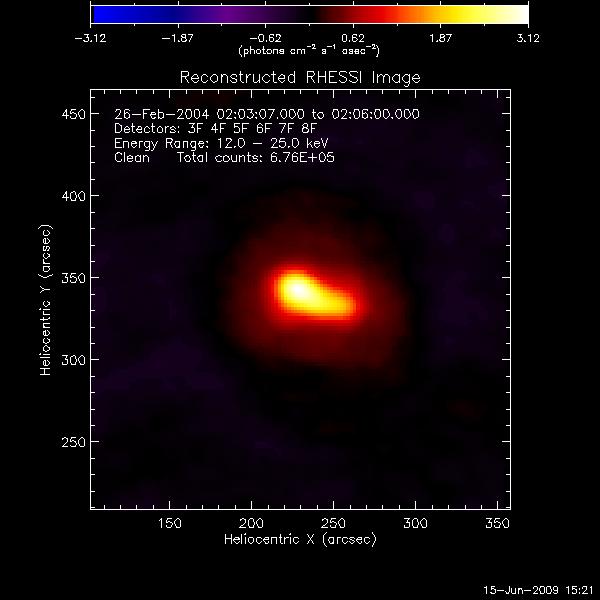
have enough counts to make images
for energy intervals 6-12 Kev, 12-25 Kev, and barley enough for 25-50
but I made an image for it anyways.
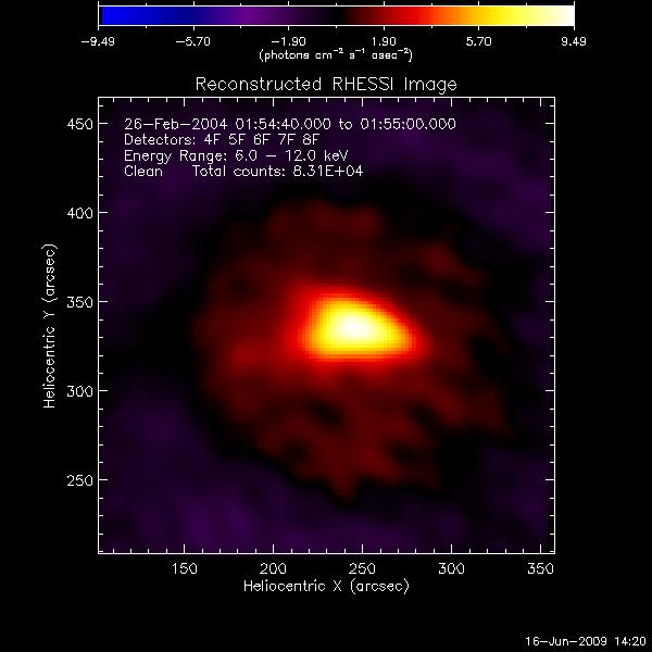
Time
start-2:03:07
Time end-2:06:00
Energy intervals-6-12
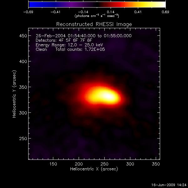
Time
start-2:03:07
Time
end-2:06:00
Energy
intervals-12-25

Time
start-2:03:07
Time
end-2:06:00
Energy
intervals-25-50

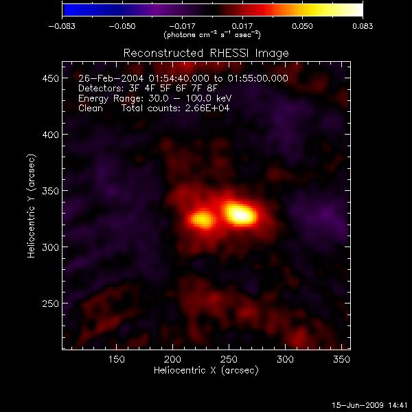
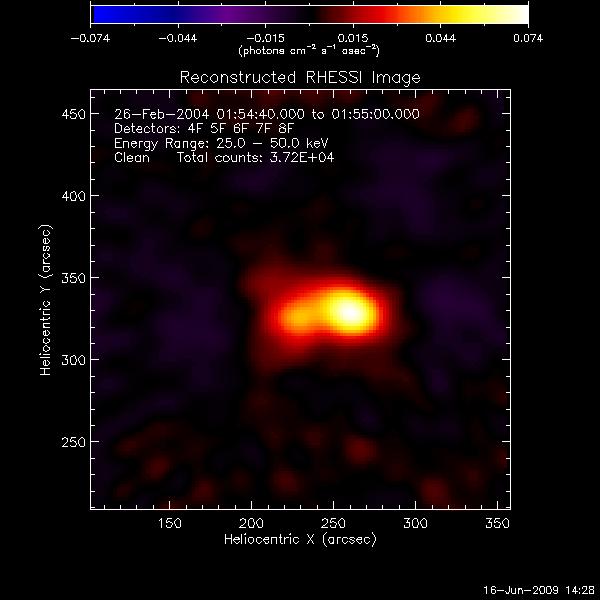
I mimicked Angela’s dissertation and
did a
RHESSI image for the beginning of the flare.
Time
start- 1:54:40
Time
end- 1:55
Energy
level- 30-100 keV

June 16,2009
I
continued to make
corrected images and graphs of my flare.
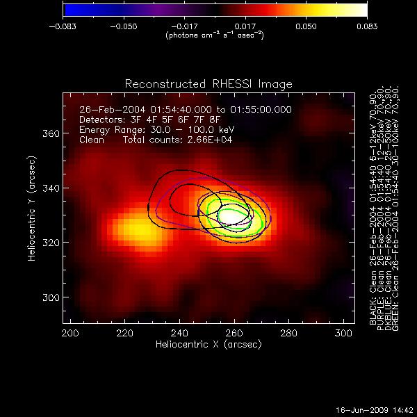
I
made an overlay of
lower energy intervals over the foot point to show
the movement of X ray flux.
Before
the overlay I had
to make RHESSI Images of each energy interval
from 6-50 keV.
Energy range: 6-12 keV

Energy
range: 12-25 keV

Energy
range: 25-50 keV

The
final product with
the overlay of the four different energy levels
including 30-100 keV.
The
contour intervals are
90 and 70 percent of the max.

I
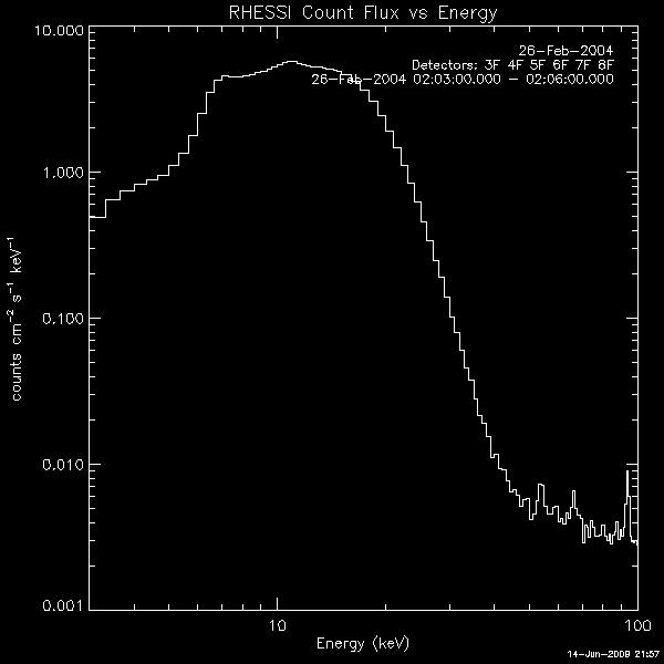
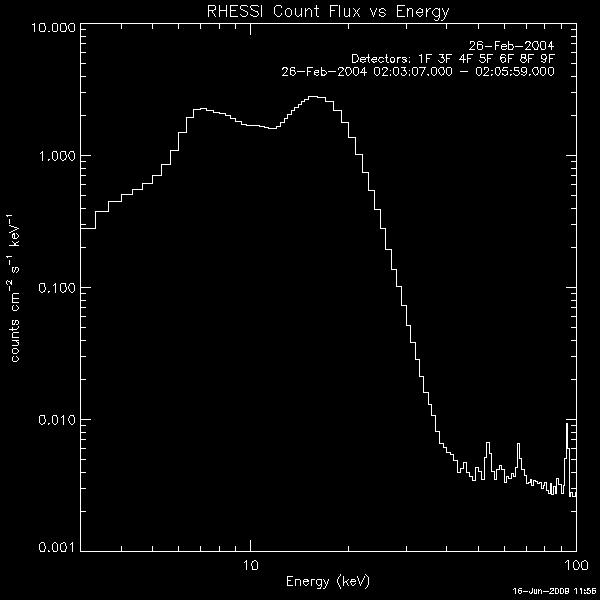
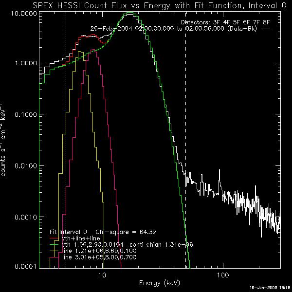
made another spectrum graph from time 2:03:07 to 2:06 because
the
original spectrum graph start at 2:03 and it was beginning an
attenuator
change. The graph did not look as clear as this one below.

I
continued to work on the second half of the
OSPEX
tutorial.
As
I was
reading I realized how important the
spectral
images are going to be
for my research
and
how this is going to be the challenging part of my
project.
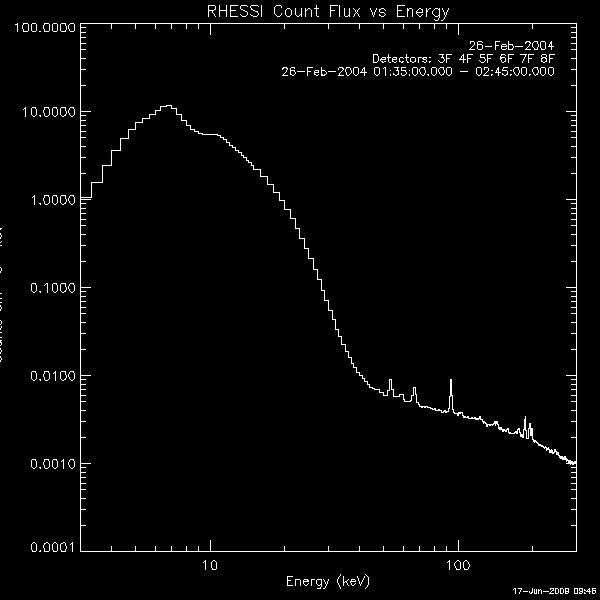
I
learned that I needed to make another spectral graph
that
included a wider range of time plus night time
up
to 50-100 keV for
background radiation.
I
continued to do the OSPEX tutorial and making notes of certain areas
that were not clear to me so I was able to pick Angela’s
brain. She made the “Fit” part of the tutorial a little
clear. Basically I will be playing with four different parameters to
make a line that will best fit the spectral in 20-sec intervals.
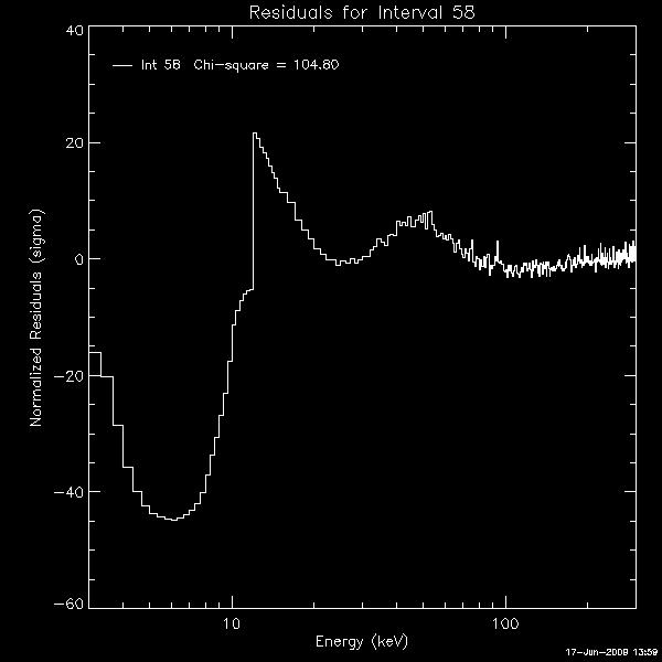
Apparently the way you can tell if each component fits the line
correctly is through a residual map which is a graph of the fit and the
chi-square helps as well.
The
different components are as follow:
Variable Thermal- optically
thin thermal bremsstrahlung radiation function as differential spectrum
seen at Earth units of photon per cm^2 s keV
2 Lines- Single Gaussian function (high) quality width in sigma
bpow- Broken Power-law function with/without
discontinuities in the derivatives.
I also realized I needed
to make another spectral image with a higher range of energy.
Energy
range- 3-300 keV

I
produced an imaged using the various components and a residual map but
I’m not too sure if it is correct. Then I made the program loop through
the time intervals starting from the one I was previously looking
at. By the end of the working day the program was still looping
so I left it running over night.


June 18,
2009
I
was interested to see if the loop was finished since I never left a
program running over night and to my surprise it was not finished. It
finally finished and I was able to finish the tutorial.
After
I spoke to Angela I learned that I didn’t have to do any looping
initially but now I know the procedure to do it. We went over
more details on how get a good fit of the spectrum. Unfortunately, the
program was cutting of my spectrum curve in the smaller time intervals
but after restarting the OSPEX GUI it proceeded to work and I was able
to ask questions. I learned how to make smaller adjustment on the
parameters of each component to get a decent fit for my curve.
For
the time being I am
to work on one time interval at a time to figure out the parameters. I
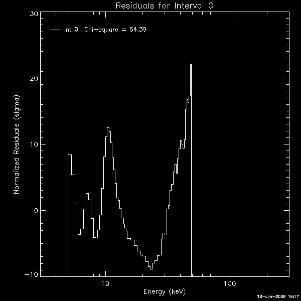
know if I have a good fit by looking at the residual graph and the
chi-square. The graph
calculates the total components and the actual data to calculate the
best fit. When there is a good fit the line on the residual graph
would have a maximum and minimum of 5 but it is centered at origin and
goes across the x axis. The chi-square value should be around one
for a good fit. The residual map below had a chi-square value of 79 and
I managed to lower its value to 64.39 (this mean it is a horrible fit).
The fit map only has the
thermal, line 1, line 2, and it is missing the broken power law
component.


June 19, 2009
I
went to an amazing lecture presented by Dana Longcope about the
radiation zone and the convection zone. The lecture gave me more
insight of how the sun is operating and creating a magnetic field.
I
met with Angela and went over the spectrum graph I produced with the
fit line and discussed the next step in the process.
-Loop other time intervals:
* with the
thermal component only
*with thermal
and broken power law component
- From the thermal component find the
relationship between the energy and temperature using the
Equipartition theorem- E= (3/2) *Kboltzman*T.
-Use two thermal components without the broken power
law after 2:05
Then
Angela and I discussed my agenda for next week in her absence.
-continue working on the spectrum graph with fit lines
-continue working on the topology overlay
- Look at the
TRACE tutorial
