Coronal Tomography with STEREO (+TRACE)
Charles Kankelborg
November 6, 2007
ABSTRACT
I will present some preliminary results on 3D coronal reconstructions from STEREO+TRACE data,
using an algorithm that is surprisingly simple. The data are all simulated at this stage,
because I need a known answer to test the algorithm (and I'm not yet ready to deal with
instrumental issues in my software!)
Introduction
- The STEREO mission
- Extreme UltraViolet Solar Imager (EUVI)
instrument
- FOV: full Sun, to 1.6 solar radii
- 1.6 arc second pixels
- Wavelengths: 171, 195, 284, 304 Angstroms (just like SOHO/EIT)
- EUVI
observations;
anaglyph movie
- Prior attempts (very little published):
- Tomographic reconstruction (why is it hard?)
- m*N^2 vs. N^3
- Analytic solution using 2 spacecraft
- Perhaps a third
view would help? TRACE observes in 171, 195, 284 from LEO.
- Enter SMART, an algorithm I developed for MOSES spectral inversions.
SMART Algorithm
SMART = Smooth Multiplicative Algebraic Reconstruction Technique.
After inventing SMART (I even had the acronym, believe it or not),
I learned that it is a close relative of an existing algorithm
with almost the same name, MART (e.g.
Takayuki 1991,
Verhoeven 1993, and references therein).
Here is how the algorithm works:
- We are given projections at 3 angles theta: Id(theta, x, z),
integrated through an unknown object O(x, y, z), on some finite domain D.
- Initial guess G(x, y, z) = 1 on D.
- Initialize undercorrection parameters, gamma(theta) = 1/3.
- Rotate G and project to form Ip(theta, x, z).
- Calculate reduced chi-squared, Xr(theta), for each theta.
- gamma(theta) = gamma(theta) Xr(theta), but ensure gamma < 1/3.
- Apply smoothing: G = G * K.
- Correction factor Crot(theta, x, y, z) = (Ip/Id), constant in y!
- Rotate Crot by -theta to form C(theta, x, y, z).
- G = G prod_theta [ C(theta, x, y, z) ^ gamma(theta) ]
- return to step 4. Iterate until Xr = 1 for all theta.
If the above does not make sense, it may help to ignore the z-dimension. z is perpendicular
to the ecliptic plane. Each value of z corresponds to an essentially independent tomography
problem, because the rotations (theta) are performed about z.
Some important points:
- Correction scheme is inherently positive.
- Smoothing also provides numerical stability.
- Feedback in step 6 ensures convergence to Xr = 1.
Dynamic equilibrium between smoothing and correction...an ideal fit to the data!
Fake Data
Why not real data? Well, real data is harder. But more importantly, when you are done
analyzing real data, you don't know whether the answer is right!
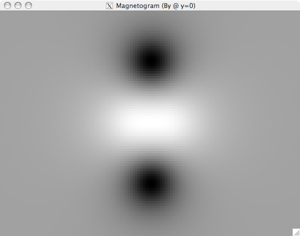
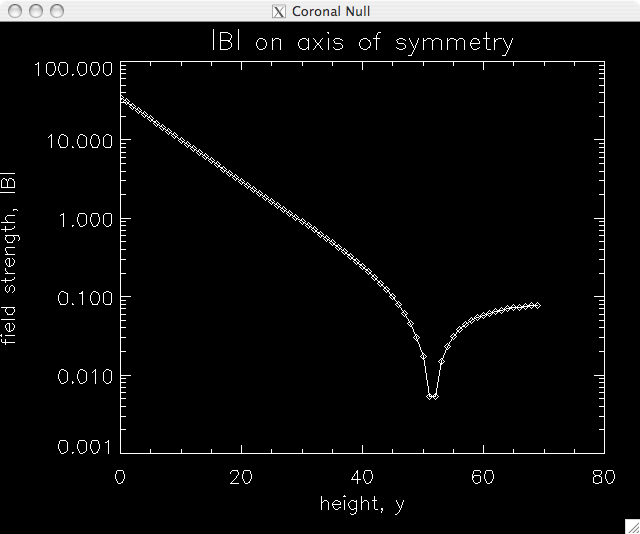
Magnetic field
- Four sub-photosphere magnetic charges.
- Coronal null.


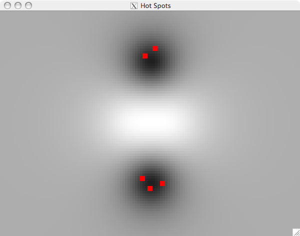
Loops
- Heated strands identified by photospheric mask.
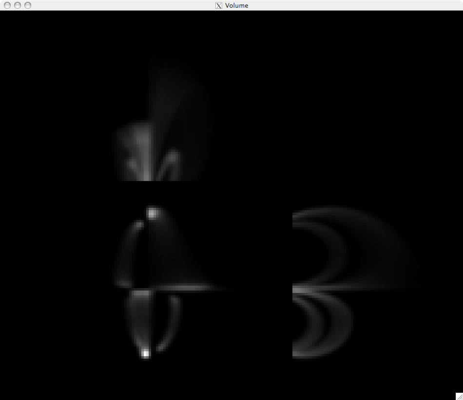
- Emissivity goes as the number of heated field lines per voxel.
- Light smoothing.


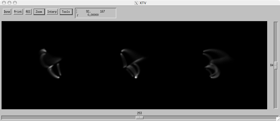
Image data
- Randomly chosen clocking angle and heliographic longitude.
- 3 projections, maximum 3000 counts.
- Poisson noise.


Results
- Number of iterations is set to 15.
- Converges to Xr=1 (usually).
- The result is not sensitive to smoothing (the only adjustable parameter).
- The solution is stable for any number of iterations after convergence.
- Computation time: a few minutes on my MacBook Pro for a 169^3
volume.
- Most or all features recovered. Minimal artifacts.
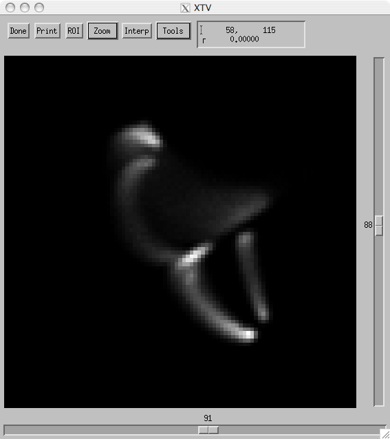
The following movies are square root scaled. They compare the original volume model (left) to the SMART
reconstruction (right).
The first three of these movies use the same volume model, with different randomly chosen
clocking angles and heliographic longitudes. The last movie started with a slightly different
magnetic configuration, with one loop that encounters the coronal null and spreads out in a
fan to the edges of the domain. This demonstrates very clearly that the algorithm can handle
arbitrary geometries, unlike previously developed algorithms for STEREO data.
Discussion
What do the results mean?
- Inversion basically works. Better than I expected!
- Even oddly-shaped structures are recovered, because there are no prior
assumptions about geometry.
- There is some blurring, which is to be expected.
- Some ghosting is visible in the reconstruction. Can be improved
if the volume is restricted to y > 0.
There is lots still to do. Next step is an ApJ letter. Perhaps a SECCHI Guest
Investigator proposal. Applying to observations is a big task!
