 |
Documentation > SXT Observation Notes > this page |
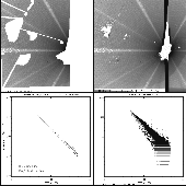
Image name: scatt_al_920906.png (click image to enlarge)
Image size: 284.468 KB (1024x1024)
Date submitted: 26-Jun-1994

SXT X-RAY SCATTERING FUNCTION (THIN ALUMINUM)
L. Acton    22-Jun-94, text corrected 26-Jun-94

This figure displays the analysis of the x-ray "starburst" image of
9-Sep-92 18:57.  The processing was done as follows:

1.  Select sfr and spr data for that orbit.
2.  Process PFI Al.1 data to derive, by interpolation of the light curve,
    the total Al.1 source intensity at 18:57.  The result was 5.7e8 DN/sec.
3.  Run SXT_PREP on the FFIs:
   0  6-SEP-92  18:30:00  QT/H  Open /Al.1  Half Norm C  23  2668.0 512x512
   1  6-SEP-92  18:48:34  QT/H  Open /Al.1  Half Norm C  23  2668.0 512x512
   2  6-SEP-92  18:50:42  QT/H  Open /AlMg  Half Norm C  23  2668.0 512x512
   3  6-SEP-92  18:57:06  QT/H  Open /Al.1  Half Norm C  23  2668.0 512x512
   4  6-SEP-92  18:59:14  QT/H  Open /AlMg  Half Norm C  23  2668.0 512x512
   5  6-SEP-92  19:03:30  QT/H  Open /Al.1  Half Norm C  23  2668.0 512x512
IDL> sxt_prep,index,data,iout,dout,/register,ref_image=4,/roll_do,/interp,$
IDL> /dc_interpolate,outres=1
4.  Form the image shown in upper right by subtracting dout(*,*,0) from
    dout(*,*,3).
5.  Determine the flare source location by the location of convergence of
    the spider rays.  The result was:  x0=404, y0=232.
6.  Run my program SCAT_AVG.PRO to:
	a.  Compute the radius of each pixel from the source location.
	b.  Use WDEFROI to select the area for analysis, avoiding the
	    areas contaminated for one reason or another.  (The area used
	    to derive the scattering function is shown in the upper LH image.)
	c.  Plot the signals vs radius for the selected area. (Lower RH plot.)
	d.  Normalize the signals by dividing by the source intensity.
	e.  Divide the data into radius bins and form averages.
	f.  Plot these average values vs. radius.
	g.  Do a linear fit of log(avg signals) vs. log(r).
	h.  Overplot that fit.
	i.  Output to the screen the fit parameters and the scattering function.

The result of this process is the following equation:

	Yscat = 0.00168*R^(-1.89)   per HR pix, with R measured in HR pix.

The lower LH panel shows the averaged, normalized signals, equation 4 from
the Hara coronal hole paper, and the LWA/JLC fit of 7-Jun-94 (taken along a
single ray 5 degrees above the horizontal).

Note that there is considerable radial structure in the scattered signal.
I have computed the slope for a number of rays, avioiding the spider
shadows, and find values ranging from about 1.7 to 2.1.  I believe the
grand average given here is about as good as we can do to represent
this scattering for data analysis -- assuming that this image is
characteristic of the general case.  A similar analysis should be done for
other starburst images, and for AlMg, for comparison.