Hinode/XRT response functions

XRT temperature response with other choice of abundances.

(April, 2011 by Aki Takeda)
(June, 2011 revised.)
(July, 2011 revised.)
(September, 2011 revised.)
(November, 2011 revised: added compariton between Chitnai 6.0.1 and 7.0)
(April, 2012 revised.)
(January, 2013 revised.) added plots of effective area function.
(February, 2013 revised: added compariton between Chitnai 6.0.1 and 7.1)
(February, 2014 revised: added compariton between Chitnai 6.0.1 and 7.1.3 and between old/new filter calibration.)

1. Introduction.

Current official XRT temperature response assumes " coronal" abundance, and calculated with Chianti 6.01. However, the temperature responses and the resulting filter ratios are affected by the choice of abundance. There are a few sets of abundances proposed in the literature.

(a) Coronal abundances based on Feldman et al. (1992) ApJSS, 81,387.
(b) Hybrid abundances base on Fludra & Schmelz (1999) A&A, 348,286.
(c) Photospheric abundances base on Grevesse et al. (2007) Space Sci. Rev.,130, 105

2. The response functions with other abundance.

To calculate the XRT response functions, I calculated the solar spectra with different sets of elemental abundances other than 'coronal'. Those spectrum files are currently stored in ~takeda/idlpro/xrt/xrt_resp/solar_spectrum.

(a) solspec_ch601_corona_chianti.genx
(b) solspec_ch601_hybrid_chianti.genx
(c) solspec_ch601_photos_chianti.genx

Link to these spectral files.
Then I modified XRT_FLUX.PRO so that it can access the above spectrum files by setting the corresponding keyword.
(~takeda/idlpro/xrt/xrt_flux.pro) IDL> flux_c = xrt_flux(logte, f1,f2, tim, /corona) IDL> flux_h = xrt_flux(logte, f1,f2, tim, /hybrid) IDL> flux_p = xrt_flux(logte, f1,f2, tim, /photos) IDL> flux_ac = xrt_flux(logte, f1,f2, tim, /apac) ; this KW is available since the original version.

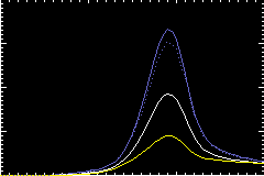
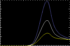
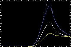
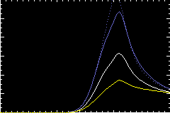
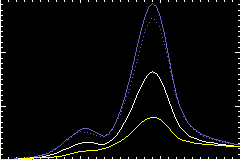
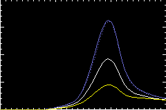
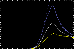
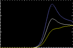
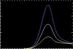
Below are the response functions of all the X-ray analysis filters available at XRT (cf: their effective area functions). The calibration data released on 20-Aug-2010 was used for these calclation. It is known that the contamination accumulated on the CCD modifies the XRT response functions. As the amount of contamination varies with time, response functions are time-dependant. For the later convenience of analysis, the following response functions were calculated for the contamination level as of 12-Nov-2006.
Plots are clickable (i.e., click each plot to show more detailed info).

Al-poly/Open	C-poly/Open	thin-Be/Open	med-Be/Open	med-Al/Open

Open/Al-mesh	Open/Ti-poly	Open/thick-Al	Open/thick-Be	Al-poly/Ti-poly

In response to the release of Chianti version 7.1.3 (August, 2013) and the recalibration of the XRT filters (made available in November, 2013), the XRT response functions were re-calculated using the latest version of atomic data and XRT new effective area functions. The comparison plots were prepared in this page.

The comparison plots of Chianti 7.1 and 6.0.1 are now moved this page.

The comparison plots of Chianti 7.0 and 6.0.1 are now moved here.

3. The Filter Ratios.

When the XRT observed the isothermal plasma (with the temperature, T) along the line of sight, the expected data number (DN) per unit emission measure (EM) has the form,

DNi=Fi(T)xVEM.

Here, i denotes different filter, VEM is the volume emission measure, and Fi(T) includes the information of the solar spectra and telescope's spectral response, integrated over the wavelenth. Assuming the same volume of plasma is responsible for the emission observed with the both filters, the ratio of the DNs obtained with different filter becomes only depends on the temperature, T (i.e., T is derived from the filter ratio). Below are the filter-ratio plots of 14 selected pairs.
Again, plots are clickable (i.e., click each plot to show more detailed info).

C-poly/Al-poly	thin-Be/Al-poly	med-Be/Al-poly	med-Al/Al-poly	thin-Be/C-poly

med-Be/C-poly	med-Al/C-poly	med-Be/thin-Be	med-Al/thin-Be	med-Al/med-Be

Al-poly/Al-mesh	Ti-poly/Al-mesh	med-Al/Ti-poly	thick-Be/med-Al	Ti-poly/Al-poly

thin-Be/Al-mesh	thin-Be/Ti-poly	thick-Be/thick-Al	thick-Al/Ti-poly

As you can see from the above plot, the filter pair, med-Al/med-Be, shows odd behavior in the following two points. (1) the ratio is decreasing over 6.3MK. and (2) Below 6MK, the ratio exceeds 10^10 due to relatively higher response in med-Al fileter for this range. (in the above plot, the part is not shown). The med-Al/thin-Be pair also shows the tendency (2).

3. Test analysis of an active region (AR10923).

AR10923 : observed 12-Nov-2006 in all FW1 filters, i.e., Al-poly, C-poly, thin-Be, med-Be, and med-Al (all with FW2 is Open). This region was studied in the following papers.

Reale et al. (2007) Science, 318, p.1582
Reale et al. (2009) ApJ, 698, p.756
Parenti, Reale, and Reeves (2010) A&A 517, A41

Figures from Reale et al. (2009).

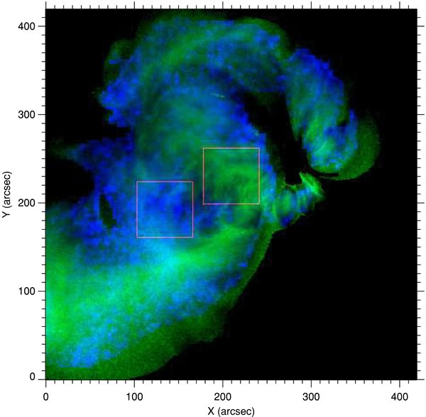
[left] Maps of temperature as in Figure 2 obtained with CIFR (green scale) and hard (F4/F5) filter ratio (blue scale). The red boxes mark the regions of different temperature regimes analyzed separately: the one on the left is hotter in the hard filter ratio (hereafter hard-hot region), and the one on the right is hotter in the soft filter ratios (hereafter soft-hot region).

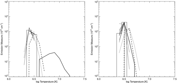
[right] Emission measure distributions vs. temperature for the hard-hot (left) and soft-hot (right) subregions marked in the temperature map. soft filter ratios (thin solid lines), CIFR (histogram), F5/F3 (dotted line), F4/F3 (dashed line), F4/F5 (thick solid line). The latter is obtained from the map binned over boxes of 4x4 pixels.

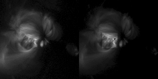
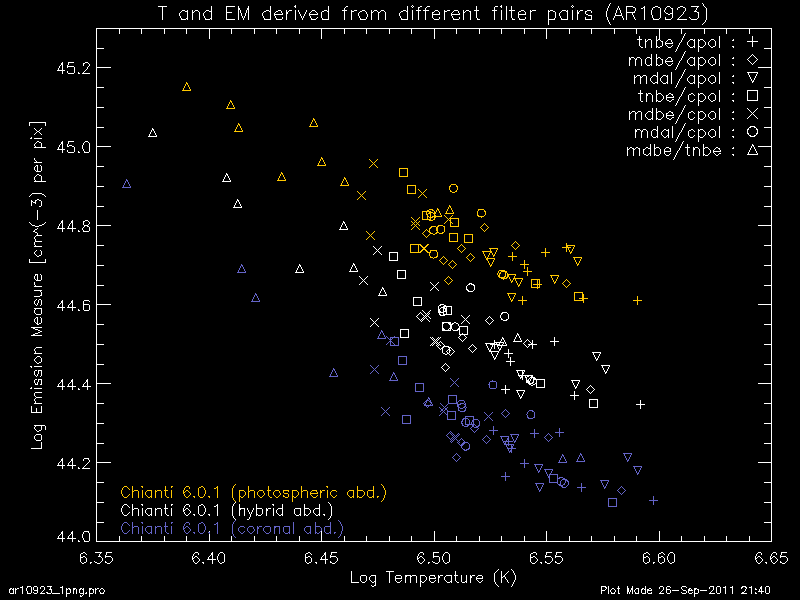
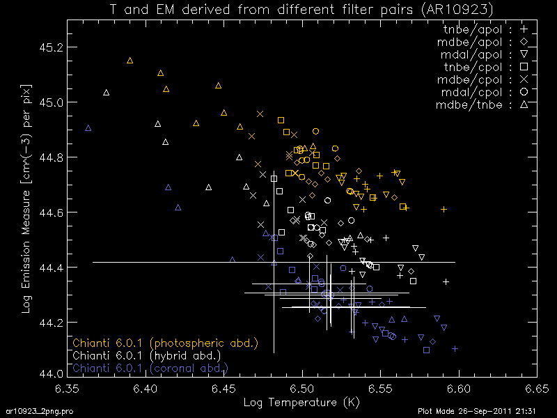
The analysis so far I made.

Get data for 12-Nov-2006, 13:00 -- 14:00.
12 sets of 512x512 images, in Al-poly, C-poly, thin-Be, med-Be, and med-Al.
Confirmed no night, no SAA, no significant activity (GOES B0 level).
No significant jitter, was in pretty stable pointing.
PREP IDL> xrt_prep,index,data, iout,dout, /norm,/float ; to check DN values IDL> xrt_prep,index,data, iout,dout, /float ; to pass to XRT_TEEM
Estimated systematic(photometric) errors with XRT_REL_UNC IDL> rel2_unc=fltarr(size(data,/dim)) IDL> for i=0,n_elements(index)-1 do rel2_unc(*,*,i)=xrt_unc_rel(index(i),data(*,*,i)) IDL> sysunc_tot=sqrt(rel2_unc*dout^2)
Te-EM analysis with XRT_TEEM
I modified XRT_TEEM.PRO so that it can use different abundance files. IDL> xrt_teem,i_cpol,dsum_cpol,i_apol,dsum_apol,te,em,uncte,uncem,/no_thres, /corona ; (default) IDL> xrt_teem,i_cpol,dsum_cpol,i_apol,dsum_apol,te,em,uncte,uncem,/no_thres, /hybrid IDL> xrt_teem,i_cpol,dsum_cpol,i_apol,dsum_apol,te,em,uncte,uncem,/no_thres, /photos
Separate into each wavelength.
Pick a 100x100 region similar to Reale et al (2009).
Pick a 3x3 region (X-mark) to demonstrate the DN values and errors.
TEEM analysis with modified XRT_TEEM.PRO. Get Te, Em, te_unc, em_unc without binning.
Evaluation of the obtained uncertainty.

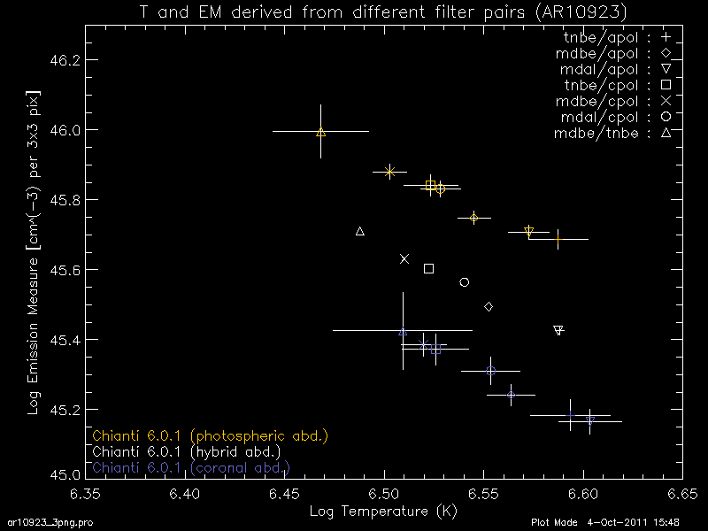Variation of the DN values of the 3x3 region.

-------  DN (preped, not normalized) ------- -- for 3x3 area total --
[Apol]  1078.37      1014.80      878.390
        946.328      919.437      885.637            10384.9
        823.303      832.155      744.774

[Cpol]  1161.43      1063.03      955.662
        939.651      889.639      870.666            10924.6 
        773.045      770.976      757.631

[tnBe]  1167.83      1077.90      1012.66
        968.508      953.946      921.393            11906.1
        905.210      875.589      771.014

[mdBe]  1216.49      1206.19      1126.13
        963.722      997.906      975.759            12734.1
        878.712      874.954      789.240

[mdAl]  1225.66      1163.70      977.267
        961.439      922.979      894.334            12213.0
        868.930      868.610      778.027

-------    DN/sec (normalized)      -------
[Apol]  4187.40      3940.55      3410.85
        3674.66      3570.24      3438.99
        3196.94      3231.32      2892.01

[Cpol]  3193.54      2922.99      2627.75
        2583.73      2446.21      2394.04
        2125.62      2119.93      2083.23

[tnBe]  807.997      745.771      700.634
        670.089      660.013      637.490
        626.294      605.799      533.447

[mdBe]  148.479      147.221      137.450
        117.627      121.799      119.096
        107.251      106.793      96.3307

[mdAl]  74.8024      71.0210      59.6430
        58.6770      56.3298      54.5815
        53.0312      53.0116      47.4833

---  systematic(photometric) errors (DN) ---
[Apol]  2.75752      2.61640      2.31510
        2.46396      2.40572      2.33055
        2.19592      2.21637      2.02755

[Cpol]  2.94353      2.72338      2.48403
        2.44941      2.34072      2.29797
        2.08799      2.08517      2.05476

[tnBe]  2.95808      2.75682      2.61040
        2.51290      2.48167      2.40903
        2.37374      2.31013      2.08348

[mdBe]  3.06783      3.04511      2.86384
        2.50242      2.57866      2.52878
        2.31615      2.30892      2.12200

[mdAl]  3.08861      2.94916      2.53230
        2.49689      2.41328      2.34939
        2.29498      2.29498      2.09845

---  photon noise (DN) ---
[Apol] 65.397878       63.248253       59.605890
       60.720222       59.979558       58.892086          204.76752
       57.276355       57.188295       53.963870

[Cpol] 67.205540       64.410526       61.642154
       60.769943       59.619345       58.821530          209.62271
       56.599102       56.169273       54.418720

[tnBe] 67.390658       64.859207       63.453673
       61.696039       61.736524       60.510796          218.83662
       61.246569       59.858847       54.897265

[mdBe] 68.960055       69.078785       67.264151
       60.690414       62.190989       61.598519          225.15279
       58.252655       58.034692       55.164978

[mdAl] 70.219142       68.491790       62.548143
       61.388868       60.061200       59.164154          223.58163
       58.633975       58.544121       55.413010

---  Temperature from [tnBe/Cpol] (in log T scale) ---
       6.4822430       6.4860326       6.5083689
       6.4935236       6.5156858       6.5075720          6.5258449
       6.5792920       6.5530505       6.4876823

---  Temperature uncertainty from  [tnBe/Cpol] (in log T) ---
       5.4306889       5.4662425       5.5823558
       5.5265759       5.6241566       5.5997766          5.1176159
       5.8922127       5.8026431       5.5470261

---  Emission Measure from [tnBe/Cpol] (in log EM scale) ---
       44.507617       44.460207       44.359245
       44.389846       44.308431       44.321024          45.372343
       44.100949       44.160929       44.309319

---  Emission Measure unvertainty from [tnBe/Cpol] (in log EM) ---
       43.945477       43.925888       43.895490
       43.900404       43.871840       43.876275          44.408615
       43.800354       43.825653       43.852398