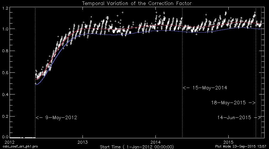
There was another increase of the visible stray light on 14-June-2015 around 12UT, indicating the 2nd rupture at another sector of the XRT pre-filter. This requires another type of correction to be applied for the data after 14-June-2015, i.e., the stray light status entered a new phase. We will use the following terms to distinguish these different status.

k0=pl8coef(0)            $   pl8coef(0)=   2.5407783
      +tt^1*pl8coef(1)   $   pl8coef(1)=  -0.050755524
      +tt^2*pl8coef(2)   $   pl8coef(2)=   0.00047431645
      +tt^3*pl8coef(3)   $   pl8coef(3)=  -2.1150909e-06
      +tt^4*pl8coef(4)   $   pl8coef(4)=   5.2729766e-09
      +tt^5*pl8coef(5)   $   pl8coef(5)=  -7.7550661e-12
      +tt^6*pl8coef(6)   $   pl8coef(6)=   6.6840085e-15
      +tt^7*pl8coef(7)   $   pl8coef(7)=  -3.1217268e-18
      +tt^8*pl8coef(8)   $   pl8coef(8)=   6.0986076e-22
Like the previous version, the offset value of -0.05
(shifting downward) was applyied as the final value of the correction
factor (blue line), in order to avoid negative values due to
over-correction.
k = k0 - 0.05These k values are not precise but give convenient way of removing the stray light component from the contaminated X-ray images. They are good enough for correcting the browse images, i.e., PNG version of the SCIA images. For quantitative analysis, however, users need to interporate the raw data points to get the proper value corresponding to the time of observation.
Comparison of New & Old fitting curves.
The PNG version of the SCIA images after 1-Jan-2014 (till 14-Jun-2015)
were re-processed using the new correction factor.
IDL> print,get_slcorfact('9-may-2012 18:00')
      0.49000561
IDL> print,get_slcorfact('15-may-2014 18:00')
      0.97750095
IDL> print,get_slcorfact('1-may-2012 00:00')
*** the input time before [9-may-2012] set to 0.
2012/05/01 00:00:00.000
      0.00000
IDL> print,get_slcorfact('1-mar-2015 00:00')
       1.0142173
IDL> print,get_slcorfact('1-jul-2015 00:00')
*** the input time after [14-jun-2014, 12UT] set to 1.
2015/07/01 00:00:00.000
      1.00000
2) RD_SLCORFACT_RAW.PRO : Provide raw data points
(returns '+' sign points).
IDL> rd_slcorfact_raw,index,factor
% Compiled module: RESTGEN.
INDEX           STRUCT    = -> MS_181626989002 Array[2189]
FACTOR          FLOAT     = Array[2189]
IDL> utplot, index.date_obs,factor,psym=1  ; to give the above plot
Here is a list of the k-factor raw values.