(20th August, 2014 by Aki Takeda)
(28-Jan-2015: correction factor part added.)
(3-Mar-2015: correction factor polynomial fitting added.)
(22-Sep-2015: plot and fitting of the factor corrected.)
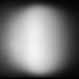
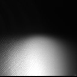
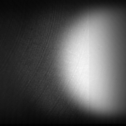
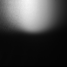
The visible stray light component contaminated in the X-ray filter images
were measured during the eclipse season of 2014.
Introduction to the stray light in XRT
| timeline No. | date & time | link to the page | purposes |
| 1 | 6-May-2014, 17:50UT | to the 1st test page | collects light curve, Ti-poly (250msec) at Dick Center |
| 2 | 15-May-2014, 18:20UT | to the 2nd test page | light curve, Ti-poly (1.4 sec) & Al-mesh (707msec) at DC |
| 3 | 27-May-2014, 20:30UT | to the 3rd test page | light curve, Al-poly (1.0 sec) & C-poly (1.41 sec) at DC |
| 4 | 3-Jul-2014, 18:30UT | to the 4th test page | light curve, Ti-poly (1.4 sec) & Thin-Be (2.83 sec) at DC |
| 5 | 30-Jul-2014, 18:30UT | 5th and 6th test page | light curve, Med-Al (32 sec) at DC |
| 6 | 31-Jul-2014, 15:49UT | light curve, Med-Be (24 sec) at DC | |
| 31-Jul-2014, 17:27UT | light curve, Thick-Al (64 sec) at DC | ||
| 1-Aug-2014, 16:26UT | light curve, Thick-Be (64 sec) at DC | ||
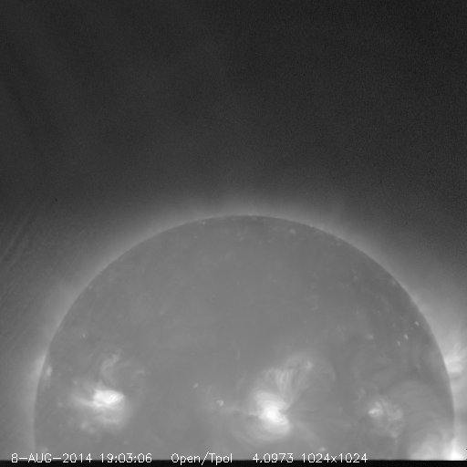
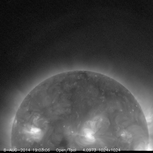
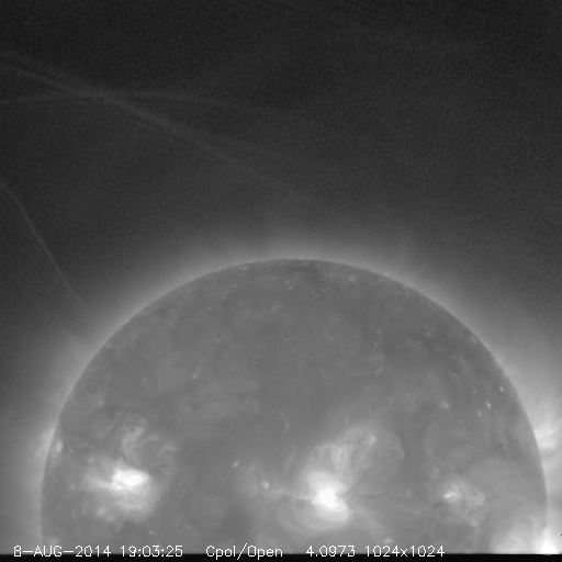
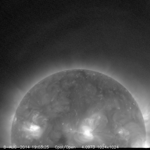
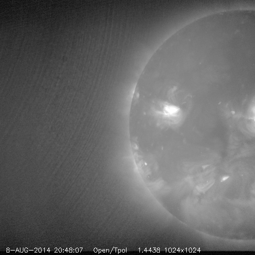
| 7 | 8-Aug-2014, 18:56UT | to the 7th test page | light curve, Ti-poly (4.0 sec) & C-poly (4.0ec) at N-pole |
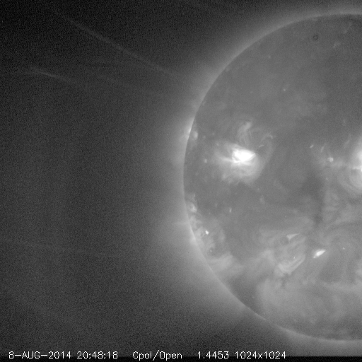
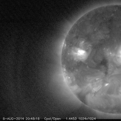
| 8-Aug-2014, 20:40UT | light curve, Ti-poly (1.4 sec) & C-poly (1.4 sec) at E-limb | ||
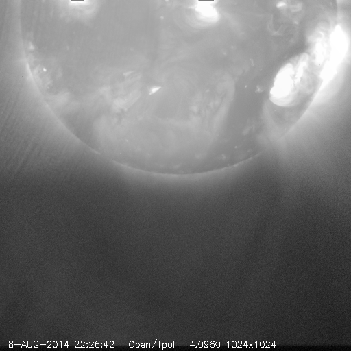
| 8-Aug-2014, 22:30UT | light curve, Ti-poly (4.0 sec) & C-poly (4.0 sec) at S-pole |
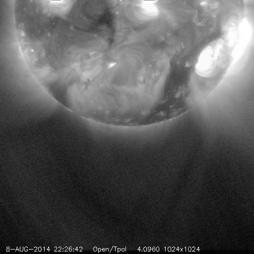
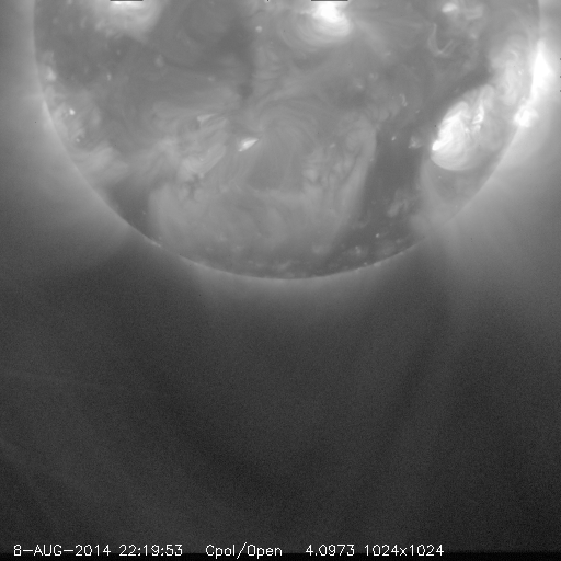
| Disk Center pointing | North Pole pointing | East Limb pointing | South Pole pointing |
 |
 |
 |
 |
| XRT20140515_182503.4.fits | XRT20140808_191124.0.fits | XRT20140808_205020.5.fits | XRT20140808_222905.4.fits |
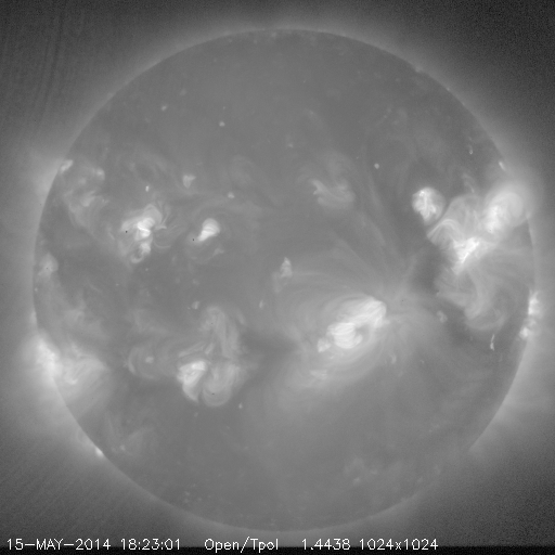
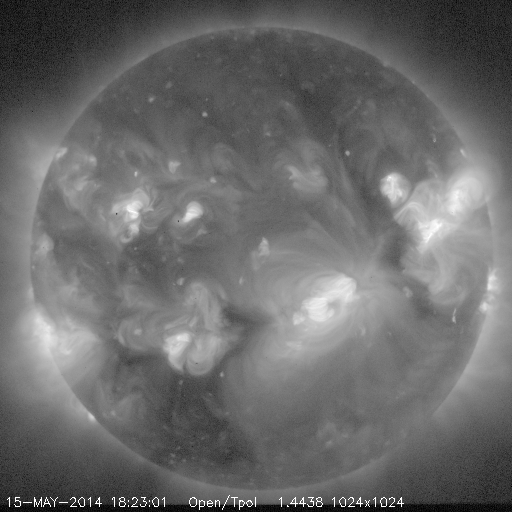
Movie of all stray-light images in Ti-poly
| Disk Center pointing | North Pole pointing | East Limb pointing | South Pole pointing |
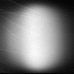 |
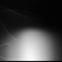 |
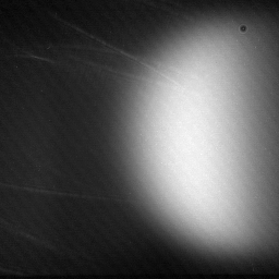 |
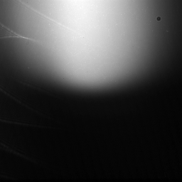 |
| XRT20140527_204601.0.fits | XRT20140808_191137.1.fits | XRT20140808_205031.0.fits | XRT20140808_222918.5.fits |
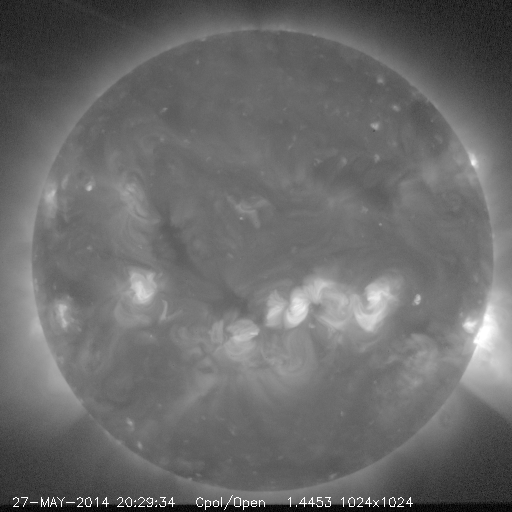
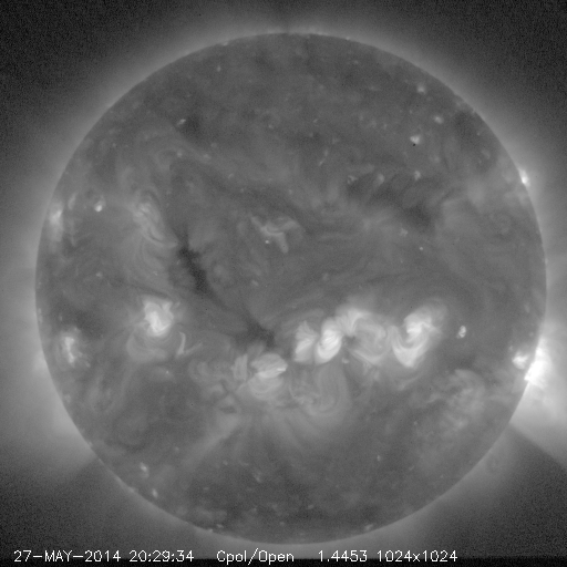
Movie of all stray-light images in C-poly
IDL> dir_l0='/disk/data/HINODE/xrt/level0/'
IDL> file=dir_l0+'2014/05/15/H1800/XRT20140515_182503.4.fits' ; T-poly stray-light image at DC pointing
IDL> mreadfits,file,index,data
IDL> xrt_prep,index,data,i_stray,d_stray,/norm,/float,/desp

; img_before : an image to be corrected, 1024x1024, Ti-poly, at DC poining, PREPed, intensity normalized.
; img_after  : an image after correction.
; d_stray    : the stray-light image prepared in the above.

IDL> img_after = img_before - d_stray
| BEFORE [synoptic (triple) composite image] | AFTER [stray light image (prep-ed) subtracted] |
 |
 |
| BEFORE [synoptic (double) composite image] | AFTER [stray light image (prep-ed) subtracted] |
 |
 |
| BEFORE [synoptic (double) composite image] | AFTER [stray light image (prep-ed) subtracted] |
 |
 |
| BEFORE [(double) composite image before twilight] | AFTER [stray light image (prep-ed) subtracted] |
 |
 |
| BEFORE [(double) composite image before twilight] | AFTER [stray light image (prep-ed) subtracted] |
 |
 |
| BEFORE [(double) composite image before twilight] | AFTER [stray light image (prep-ed) subtracted] |
 |
 |
| BEFORE [(double) composite image before twilight] | AFTER [stray light image (prep-ed) subtracted] |
 |
 |
| BEFORE [(double) composite image] | AFTER [stray light image (prep-ed) subtracted] |
 |
 |
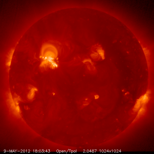
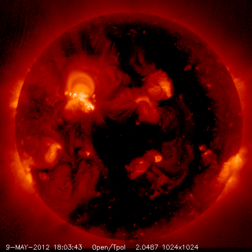
| synoptic (triple) composite image | stray-light image subtracted | stray-light image * 0.5 subtracted |
 |
 |
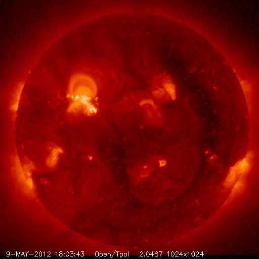 |
The stray-light is increasing:
the intensity on 9-May-2012 is about half of that on 15-May-2014.
In order to correct the images in the past (or outside eclipse season),
we need to know the temporal variation of the stray light intensity
(from 9-May-2012 to present).
[image_corrected] = [Image_uncorrected] - factor(k) * [stray-light_2014]The first rough estimation of the correction factor applied to the initial PNG products was as follows (shown in the green line in the plot below) :
k = 0.5 (9-May-2012 18:00 through 14-Aug-2012 23:59)
k = 0.7 (15-Aug-2012 00:00 through 31-Dec-2012 23:59)
k = 1.0 (1-Jan-2013 00:00 and onward)
More reasonable value of the factor is determined by using intensity correlation between Al-mesh and Ti-poly images. Note that Al-mesh images are not affected by the stray-light.
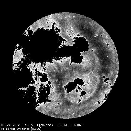
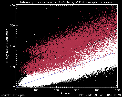 |
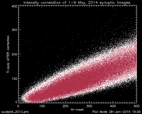 |
| White: Pixels from 1-May-2014 6UT to 9-May-2014 6UT,
masked synoptic images. Blue line: linear fit (by LADFIT, yy=2.451+0.341*xx). Red (left): 9-May-2014 18UT image BEFORE correction, Red (right): AFTER correction with the correction factor of 0.5. | |
The temporal variation of the factor k, determined by the above steps 1-6 are shown with '+' signs in the plot below (see the next subsection for the red and blue lines).
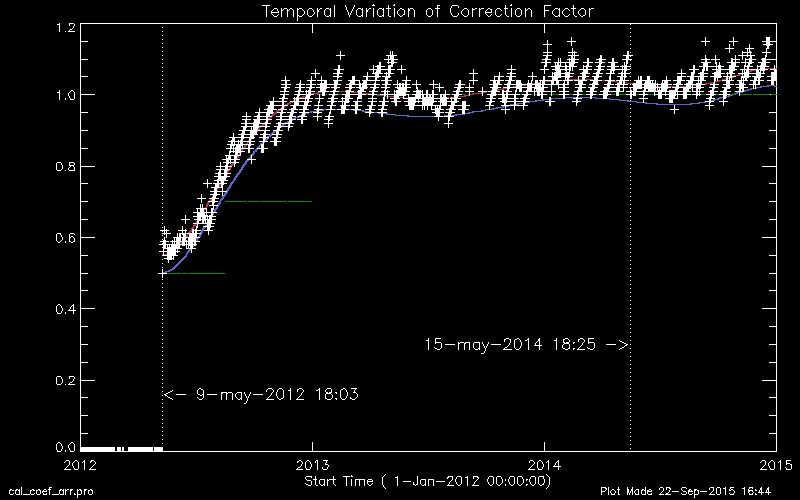
5.2 Fitting the variation of the factor, k.
[NOTE]
This sub-section(5.2) has a new version
in which the fitting was re-done using the whole data in phase 1
(9-May-2012 through 14-Jun-2015).
[NOTE]
The above data points are determined for the Al-mesh and Ti-poly pairs, each of the pair image are 'intact' (i.e., with no saturation nor telemetry drop). However, some of the intact Ti-poly images that do not have the Al-mesh counterpart are not included.
Applying the polynomial fit (7th order) to the data points between 9-May-2012 and 31-Dec-2014 (red line in the above plot).
k0 = pl7coef(0)           $    ; pl7coef(0)=   2.1924060
       +tt*pl7coef(1)     $    ; pl7coef(1)=  -0.040220413
       +tt^2*pl7coef(2)   $    ; pl7coef(2)=   0.00035595453
       +tt^3*pl7coef(3)   $    ; pl7coef(3)=  -1.4460938e-06
       +tt^4*pl7coef(4)   $    ; pl7coef(4)=   3.1434595e-09
       +tt^5*pl7coef(5)   $    ; pl7coef(5)=  -3.7773749e-12
       +tt^6*pl7coef(6)   $    ; pl7coef(6)=   2.3664218e-15
       +tt^7*pl7coef(7)        ; pl7coef(7)=  -6.0336921e-19
To avoid negative values of the faint structures due to over-correction,
the offset value of -0.05(shifting downward) was applyied as the
final value of the correction factor (blue line).
k = k0 - 0.05I made two IDL routines:
IDL> print,get_slcorfact('9-may-2012 18:00')
      0.50596564
IDL> print,get_slcorfact('15-may-2014 18:00')
      0.98621502
IDL> print,get_slcorfact('1-may-2012 00:00')
*** the input time before [9-may-2012] set to 0.
2012/05/01 00:00:00.000
      0.00000
IDL> print,get_slcorfact('1-mar-2015 00:00')
*** the input time after [31-dec-2013] set to 1.
2015/03/01 00:00:00.000
      1.00000
2) RD_SLCORFACT_RAW.PRO : Provide raw data points
(returns '+' sign points).
IDL> rd_slcorfact_raw, index,factor
% Compiled module: RD_SLCORFACT_RAW.
INDEX           STRUCT    = -> MS_163834261002 Array[1938]
FACTOR          FLOAT     = Array[1938]
IDL> utplot, index.date_obs,factor,psym=1  ; to give the above plot
The full-res images (2048x2048) included in the above period were also corrected by sabtracting the half-res stray light image(1024x1024) re-bined to 2048x2048.
The PNG products after Jan-2015 are tentatively corrected with the value of k=1.0. The k value will be updated in the future by a new fitting applied to the new data.