Relating The Physical Properties of Active Regions to Solar Flares
Abstract:
In this report I will discuss the procedure and results obtained
in trying to relate characteristics of active regions to the flare production
of those regions. The method we used was statistical. We compared
characteristics and flare data from over 120 regions. We considered the
alpha value for the region, Bz, |Bz|, Jz, (where B is the magnetic field and J
is the current) and the perpendicular magnetic field and the total
magnetic field. In considering flare production we looked at the integrated
energy flux released by the flares, the size of the maximum flare, and
the number of flares produced. We concluded that there is no relation
between the alpha distribution and flare production, and that the best
correlation is for the mean and variance of |Bz| with the integrated flare
energy flux. As for alpha, further investigation into its relationship with the
flare production of active regions showed that the change in the variance
of the alpha distribution over time is related to the flare production of
the region. However we did not find a relation between changes in alpha and individual events.Introduction:
The purpose of this project is to examine in a statistical fashion the
characteristics of active regions with measures of their flare production.
Active regions are area's on the suns surface where a strong magnetic field has
risen up out of the convection zone. These regions are often visible as
sunspots. Sometimes these regions create solar flares. These bursts of energy
out of the sun are related to the magnetic fields from which they get their
energy.
Originally it was thought that the best characteristic to look
at would be alpha, a measure of magnetic field helicity defined by the
equation:
(1)
This seems logical as one would expect that the stresses associated with the
twisted magnetic field would cause it to release energy, in the case of the sun
this would lead to solar flares. In the data we examined it did not appear
that the general alpha distribution played a role in determining the solar flare output
of the region. Thus the search for a characteristic that could correlate with
flare production was extended to Bz, |Bz|, Jz, B2 and Bperp2. In all cases
we considered the way the characteristic was distributed throughout the
active region.
We also continued to investigate the properties of alpha and how
it affects the region. In addition to the distributions of alpha we also
considered the "alpha-best", which is a best fit alpha value for the whole active
region calculated with the assumption that the magnetic field in the active region is
a linear force free field. Additionally, we looked at how these different measures of
alpha varied over time, within an active region and in a statistical sense.
The data describing characteristics of the active region was
obtained from the Haleakala Stokes Polarimeter. The data describing flare
production was obtained from GOES.HSP Data Preparation:
The HSP data was reduced by Dibyendu Nandi and Alexei Pevtsov.
Most of the data preparation and analysis was done using IDL. In
all cases the reduced HSP FITS files were read into IDL and the
magnetograms examined visually. Those magnetograms that were missing large
areas due to clouds, or appeared flawed or inconsistent with other
magnetograms were removed from the data set. Something like 50
magnetograms were removed, in most cases because a significant portion of
the magnetogram was missing, probably because of clouds.
After inspecting an image of the magnetogram to ensure it was
reliable the distributions of the desired region characteristics were
extracted. The alpha distributions were obtained through the use of an IDL
program called localalpha. This program uses the FITS data about Jz and Bz
to obtain values of alpha at each pixel and creates an array of alpha
values for the region. This is a fairly straightforward procedure because
the values Jz and Bz are already included in the FITS files and alpha can
be calclulated readily using:
(2)
In order to minimize noise only those pixels with a magnetic field above
300 Gauss were considered, this is also true for the other parameters.
The other distributions could be obtained almost directly from the
FITS data file, but they were first multiplied by the area of the pixel.
Thus the equations for these distributions are given by:|Bz|=|bz| x dA (3)
Bz = bz x dA (4)
Jz = |jz| x dA (5)
Bperp2=(bx2+by2)x dA (6)
B2=(bx2 + by2 + bz2) x dA (7)
In the above equations i use lowercase 'b's and 'j's to indicate that
these are the values that come directly from the data file. Note also,
that when I refer to |Bz| or some other quantity, I am referring to a flux
as described in (3)-(7). The dA was given in Mm^2, but had to be converted
from arcs. This was easily done using data from the FITS file that gives
the size of the sun in arcs. Since we know that the radius of the sun is
695.9 Mm, the conversion factor can be determined from the data structure.
For all the magnetograms analyzed the number of points above 300
gauss was also recorded, this turns out to be very important later on.GOES Data Preparation:
Flare data was obtained from the GOES satellites. Using the
sswidl routine pr_gev all the GOES data in the database was printed to a
file. This file was then crossreferenced with a list of all the active
regions for which we have reduced HSP data. The resulting file contained
information about maximum energy of flares, start, max and end times. The
data about number of flares, and maximum flare energy for an active region
could be obtained from this.
Probably the most interesting information about a regions flare
production was given by the integrated flare energy for the active region.
This was obtained using the GOES 3 second data, that is, GOES measures of
x-ray flux that are taken every three seconds (3.06 seconds actually).
by passing the start and end times of the flares obtained from pr_gev and
using another ssw routine called gxd_data a numerical integration over time
could be done to determine the total energy emitted by a flare. We used the
1.0 to 8.0 angstrom band of the GOES xray data for determining the energy,
which was consistent with the usual classification of flares. That is, the
1.0 to 8.0 band energy reflects the B,C,M, or X classification. The total energy
of each flare was then summed over all the flares for an active region to
determine the active regions that produced the most and least flare
energy.Analysis:
From the list of integrated flare energy by active region 120
regions were chosen, 20 of the most active and 20 of the least active as
well as 80 regions interspresed between them. For each of these regions
the distributions of alpha, Bz, Jz, etc... as well as the maximum flare
energy, number of flares, and integrated flare energy were obtained.
There were two possible ways to analyze the distributions. one
could combine all the values obtained from each pixel in all magnetograms
together to create a list of values that would form a sort of distribution for
the whole active region and calculate statistics based on that, or one could
calculate statistics for the distribution of each magnetogram and take an
average. Both methods were used initially, but we determined that doing
the statistics by magnetogram and taking an average was the best way
because using integrated statistics might have a tendency to overstate
certain statistics, such as variance. Thus for the remainder of this
paper all statistics and correlation values refer to those obtained from
averaged statistics. In the case of alpha the statistics were calculated
in two ways, one took the magnitude of the alpha from each pixel and the
other took the signed alpha from each pixel. In general the statistics
obtained using the signed alpha from each pixel were the ones that were
analyzed, unless otherwise noted. This was decided because the alpha
values by pixel formed an actual distribution and the signed value gave
the center of that distribution, whereas it seemed that using unsigned
values would distort the distribution. Also, I would note that for much of
the analysis the integrated statistics were still checked in a less
rigorous way and found to be generally consistent with the averaged
statistics.
Statistics were calculated for the distributions using IDLs moment
function, which provided values for the mean, variance, skew, and kurtosis
of the distribution. The moment function uses a simple average to find its
mean, simply adding up all the elements and dividing by the number of
elements.These statistics were then compared to the energy data using the
routine r_correlate. The r_correlate function uses Spearman's rank order
correlation. A correlation was considered to be reliable if the
confidence was around .01 or better (smaller). If a statistic correlated
with an energy parameter it could be checked using the np_fit program, which
was a way of taking out dependence on other characteristics by producing a
power to which one variable could be raised and the correlation checked
for the resulting lambda. In other words, the program would generate a p
such that lamda could be fit to the statistic with the x dependance
removed.
(8)
For instance in many cases correlations were due to a strong correlation
between Energy and the number of points in the distribution, the
dependance on the number of points could be removed and the correlation
checked without it. In this case the correlation was checked twice, in one
case the points dependence was removed and the correlation was confirmed,
in the other the other parameter was removed, leaving points, and it was
confirmed that there was no correlation.
In addition to statistics of the sort already discussed, we also
compared statistics from magnetograms before and after a solar flare.
There were very few cases to be found for which magnetograms existed
within a couple of hours before and after the start and end time of a
flare event, only 21 that seemed reasonable were found. For those 21 we
examined the statistics for alpha as well as the statistics for the mean
and variance of |Bz|.
In addition to focusing on what factors are statistically likely
to affect the flare production of an active region, we also looked more
closely at alpha's affect on flare production in a less statistical
way. The first thing that was done was to see whether the average
alpha-best value for a region correllated with different statistics from
the alpha distribution and with the regions flare energy characteristics.
In doing this, both the average of the magnitude of alpha-best and the average
of the signed alpha best were used.
Next we looked at how the alpha distribution statistics changed
over time. This was done using two different methods. One was to average
the statistics from the first few magnetograms and the last few and find
the difference, to find out how the statistics changed over time.
Regarding signs, in this process we took the magnitudes of the signed
averages obtained from the distribution, because for this analysis it was
the magnitude of the twist that mattered not so much whether it changed
direction. The other method was to find the difference between the
statistics from one magnetogram's statistics and the next and then sum up
the differences (once again we considered the absolute value of the signed
mean), in order to find out whether the statistic was going down more than
up or vice versa. In both of these methods we considered only the magnitude of
the mean and the variance of the distribution,ignoring skew and kurtosis.
Finally we plotted the mean of alpha, the variance in alpha, and
the alpha-best value over time and superimposed the time and class of
flares to see whether changes in the alpha distribution related to flare
events. This sort of analysis was done for 18 regions, 10 of which had
large energies and in which the variance had gone down, and 8 of which had
small energies and the variance went up.
In the same spirit of trying to plot a single active region's
distribution over time we also tried to plot all the active regions
distributions over time. Using the first magnetogram as time zero and
measuring time from that for each region we normalized the time and
plotted the variance and mean of alpha over time. We also tried to normalize the
variance by taking the first variance as unity and the ones after it as a
fraction of the first variance for an active region. Both of these methods,
normlized time versus variance and normalized time versus normliazed variance,
were applied to only those regions where, according to the averaging method,
the variance dropped.Results:
The original thought was that the alpha distribution should have
some statistic that was well correlated to the flare production. At first
this seemed true, with the variance statistic having a correlation with
the integrated energy with a significance of 10-5 (Figure 1), but after checking
other statistics we observed that the correlation between the number of
points and the energy has a significance of 10-11 and the correlation
between the variance and the number of points has a significance of 10-15.
If the correlation with points is removed it turned out that the variance
was no longer correlated with the integrated total energy (Figure 2) , or anything
else. For all of the alpha statistics the energy and the statistics are so
strongly correlated with the number of points in the magnetogram that the
correlations between energy and distribution statistics occured only as a
result of this correlation with points. This was true of both the
magnitude of alpha, and the signed alpha statistics.
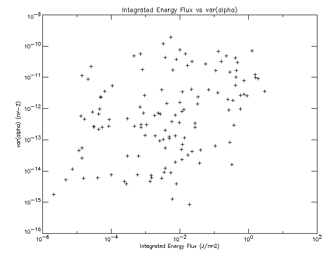
Figure 1: A plot of the variance of the alpha distribution versus the integrated energy flux. The correlation has a coefficient of 0.367586 and a confidence of 2.12485E-05.
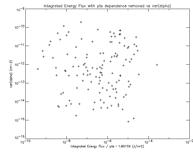
Figure 2: A plot showing the variance of the alpha distribution versus the integrated ernergy flux, but with the dependence on points removed, resulting in no correlation. (coeffiecient=.034239 and confidence=0.734199)
In examining the 'before and after' magnetograms for alpha
statistics it was found that there was no discernible pattern of
statistics changing in a uniform way from before a flare to after a flare.
Moving on to the other characteristics, it was observed that many
of the statistics there also had a strong correlation with points,
however, the variance of Bz and |Bz| as well as the mean of |Bz| appeared
to have a much stronger correlation with the energy data than they did
with the points. The best of these are the correlations were for |Bz| (Figure 3). As
for the other characteristics the correlations between distribution
statistics and energy data, were very closely related to correlations with
the number of points so that it is most likely that they are correlated
only through points and are thus unreliable characteristics.
By removing the correlation with points and then removing the
correlation with the energy data it was found that the mean and variance
of |Bz| do indeed correlate with the energy data (Figure 4).TABLE 1: correlations of |Bz| statistics and flare energy parameters.
Compare | correlation removed | value of p | correlation | significance
IntE vs. mean #Points 1.85422 0.386513 8.49856E-06
intE vs mean IntE 0.190416 0.0201781 0.823260
intE vs var #points 1.85422 0.311472 0.00040620
intE vs var IntE 0.190416 0.184909 0.0389780
maxE vs mean # points 1.25182 0.413985 1.5937E-06
maxE vs mean maxE 0.301321 -0.00712752 0.937133
maxE vs var # points 1.25182 0.323496 2.33307E-04
maxE vs var maxE 0.301321 0.462525 0.0701573
#flares vs mean # points 0.610353 0.363772 3.04567E-05
#flares vs mean # flares 0.422416 0.0672477 0.456191
#flares vs var # points 0.610353 0.322263 2.47249E-04
#flares vs var # flares 0.422416 0.215774 0.0156604The information in the table above indicates that the variance and mean of
|Bz| correlate independantly of the number of points with the integrated
energy, maximum flare energy, and the number of flares produced by an
active region.
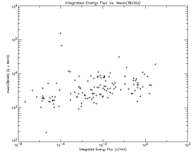
Figure 3: The mean of the |Bz| distribution versus the Integrated Energy Flux. coefficient=.485595 confidence=9.46992E-09
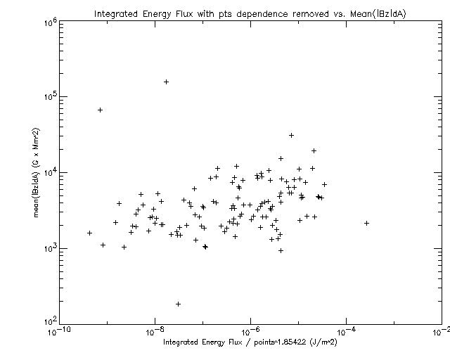
Figure 4: The mean of the |Bz| distribution versus Integrated Energy flux with the points dependence removed, showing that there is an actual correlation between the two. coefficient=.386513 confidence= 8.49856E-06
It was odd that the variance should correlate with the energy
release by the active region, so the correlation between the mean of |Bz|
and the variance of |Bz| was checked (Figure 5), it turns out that these are
extremely well correlated. This makes sense given the 300 gauss cutoff
used, if the mean is higher there will be more room for variance around
that mean than if the mean is small. This interpretation suggests that the
mean is the important correlation between |Bz| and flare energy
production.
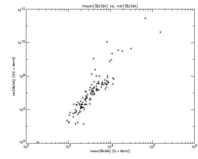
Figure 5: the variance of |Bz| versus the mean of |Bz| showing that the two are very closely correlated (so closely that when calculating the confidence the program experienced an error because the value was too small), this is probably a result of the 300 gauss cutoff used in creating the distributions.In looking at the before and after magnetograms for the 21
different flare events we found that in 15 of the events the mean dropped
after the flare, and in 16 of the events the variance dropped after the
flare. of course in the remaining events the opposite occured.
Unfortunately, 75% doesn't seem like enough for a set of only 21 events to
be considered statistically significant.
For all of the above distributions it was found that the skewness
and kurtosis of the distribution were not reliably related to the flare
energy production of the region.
The statistical analysis of the alpha-best values to the alpha
distribution values for a region turned showed that alpha-best was not
correlated with any of the distribution statistics. It also showed that
alpha-best was not likely to be correlated with the flare energy
characteristics for a region either. The best relation between alpha-best
and flare energy was with the integrated flare energy of the region, which
had a correlation coefficient of .242016 but the confidence level was only
.0316463 (Figure 6), where a confidence level around .01 or better is considered
significant. This was for the case where alpha best was calculated by
taking the absolute value of the alpha-best from each magnetogram for a
region and averaging those together to get a single alpha best for the
region.
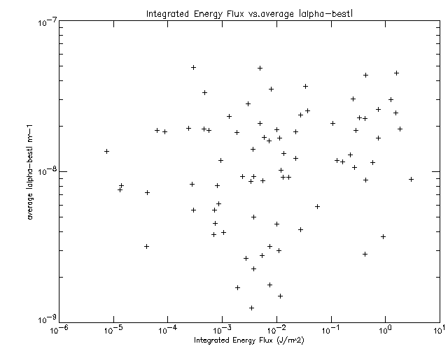
Figure 6: the average of the absolute values of alpha best for a region vs. the Integrated Energy Flux, showing a possible correlation between the alpha-best value
and Energy production. The correlation here is 0.242016 with a confidence of 0.0316463.Putting the alpha distribution statistics in chronological order
we found that about half the time the mean and variance of alpha would go
up and half the time it would go down, using either method of quantifying
the trend. It was decided to use the averaging method for the rest of the
analysis since the two methods seemed to give pretty much the same
answers. Using the averaging method a correlation was found between the
integrated flare energy production of the region and the change in the
variance of the alpha distribution. The correlation coefficient for this
relation was -.280985 with a confidence of .0105549 (Figure 7), which is fair. If the
difference method is used the correlation is still arguable, but weaker,
with a correlation coefficient of -.189822 and a confidence of .0876204.
The fact that it is detectable in both methods may be an indication that
it is an actual correlation. This correlation was also checked to ensure
that the number of points was not affecting it. As we have seen, the
number of points is related to the energy output of the region, and the
number of points is determined by the magnetic flux, so the decrease in
alpha could have been a relation with the magnetic flux instead of with
alpha, but it turns out that this is not the case. The correlation between
the change in the variance of alpha and the change in the number of points
over time had a confidence of only 0.3, implying that there is no
correlation between the two. There was no corresponding relation between the
flare energy flux of the region and changes in the mean over time (Figure 8).
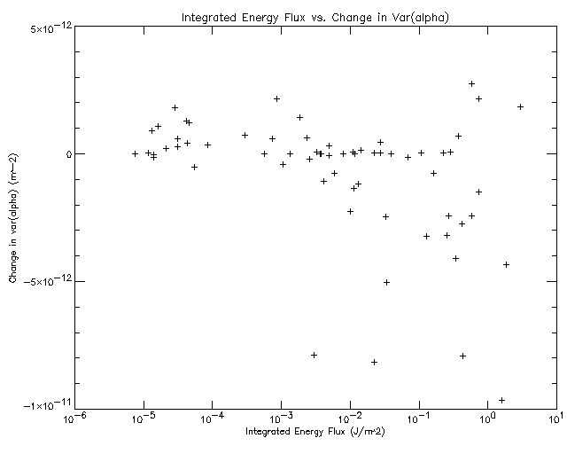
Figure 7: The change in the variance of the alpha distribution using the averaging method versus the Integrated Energy Flux, showing that there is a correlation with a coefficient of -0.280985 and a confidence of 0.0105549.
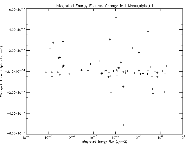
Figure 8: The change in the mean of the alpha distribution using the averaging method versus the Integrated Energy Flux, showing that there is no correlation (coefficient=-.169492, confidence=.127936).When we plotted the mean and variance of an active region over
time and indicated the times at which there were flares we found that
there may be some relation between flares and fluctuations in mean
variance and alpha-best (Figures 9 -11). It seems like in some of the plots that a concentration of
flares, or a large flare, might result in a drop in the variance. In
general the mean doesn't seem to be affected as much as the variance is,
the same seems to be true of alpha-best. It also seems like those regions
with more flares have more fluctions in both mean and variance than those
regions with less flares. However, in all cases it is difficult to say
anything conclusively, and there are many counter-examples of all of these.
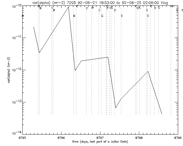
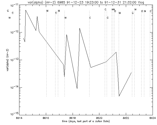
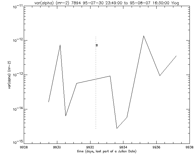
Figure 9: The variance of the alpha distribution of AR 7205, 6985, 7894 (top to bottom) over time with the times and types of flares superimposed.
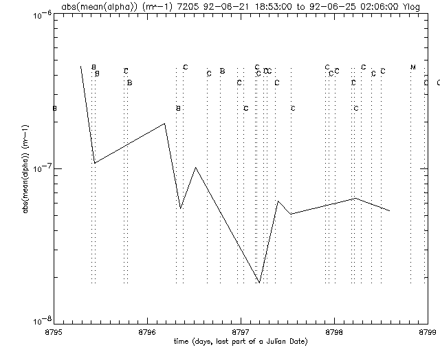
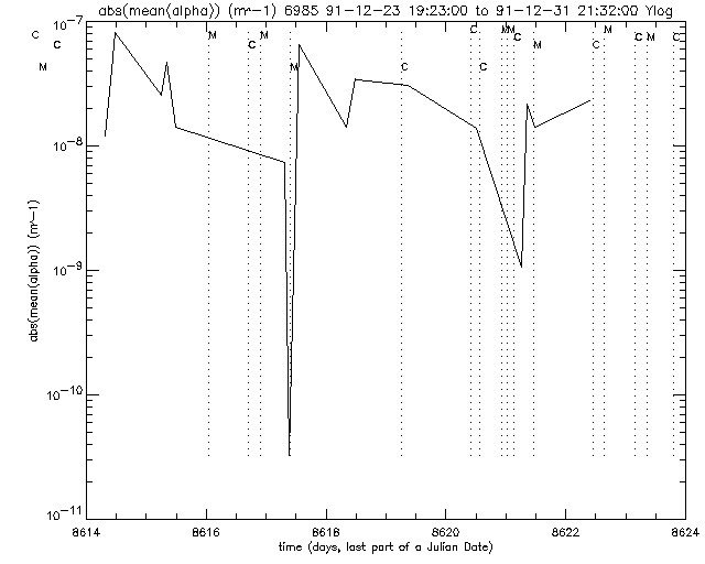
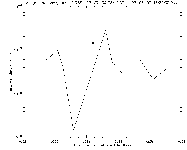
Figure 10: The mean of alpha for AR 7205,6985,7894 (top to bottom) over time, with the flares and their types superimposed.
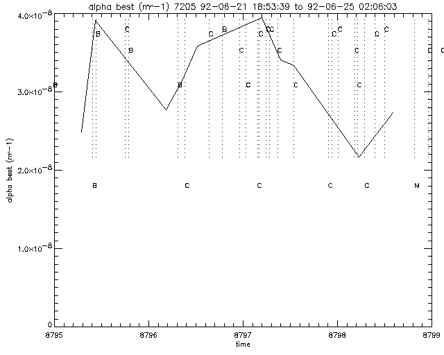
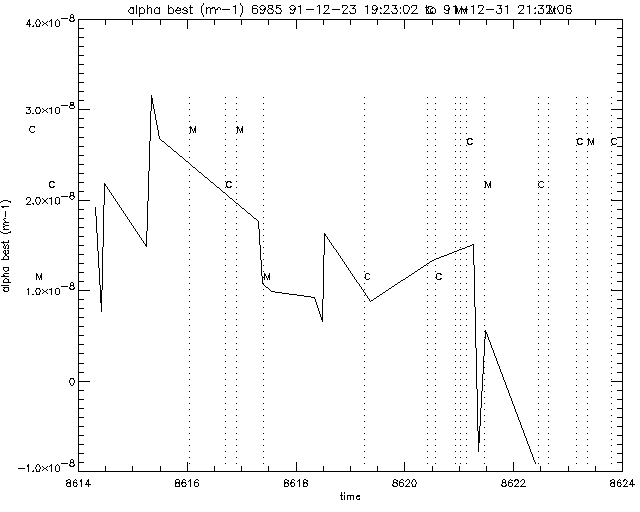
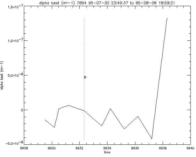
Figure 11: The alpha-best value for AR 7205,6895,7894 (top to bottom) over time with the times and types of flares superimposed.As far as plotting all the regions' mean and variance over some
normalized time there is no correlation with the variance in alpha over time,
but the mean of alpha over time has a correlation of .106783 with a confidence
of .00573412. This is only true of the signed mean, there is no correlation
between time and the absolute value of the mean. Whent his was done for
normalized variance there is also no correlation, but when it is done for only
those regions where the variance went down there is an inverse correlation
between the time since the first magnetogram and the variance of the alpha
distribution in both the real variance and the normalized variance. For the real
variance versus time the correlation was -.235783 with a significance of
1.61855E-05 (Figure 12), and for the normalized variance versus time the correlation was
-.145139 with a significance of .00709232. There was no similar relation found for
the mean of alpha going down versus some normalized time for those regions where
the variance was known to have gone down (Figure 13).
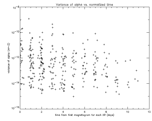
Figure 12: The variance in alpha versus normalized time (the time from the first magnetogram by active region), for only those regions in which according to the averaging method the variance went down over time. This shows that there is a correlation with a coefficient of -.235873 and a confidence of 1.01855E-05.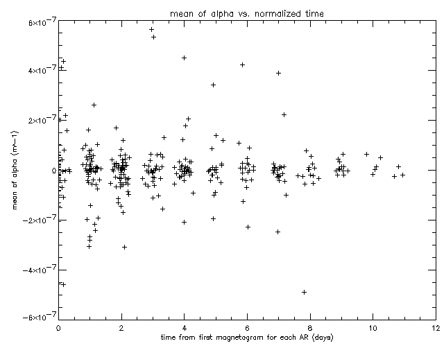
Figure 13: a plot of the mean of alpha versus normalized time for only those regions in which we know that the variance went down according to the averaging method. The plot shows that there is no corellation where the mean of alpha goes down over time (the confidence was 1.00000).
Discussion:
One concern about the method that was used here is the 300 gauss
cutoff for the pixels to be used in the analysis. I do not think this is
really a problem. For one thing the fact that the dependence on Bz can be
removed from the dependence on the number of points is an indication that
that correlation is real and so it doesn't actually matter whether we
counted more pixels or not. It is better not to count the pixels because
they would be unreliable and would introduce a great deal of noise into
the analysis. I also do not think that including more pixels would have
helped the case for correlations with alpha or anything else since the
larger energy regions also tended to have more magnetograms, so that the
correlation with points would still not be removed by including all the
points from each pixel, not to mention the additional problems that would
arise from the noise.
In any case, One thing we did determine from this investigation was
that |Bz| is related to the flare production of an active region. It makes
sense that the strength of a regions magnetic field would play a role in
determining how active it would be in its release of energy. It is
interesting that |Bz| correlates well over such a long time scale compared
to the duration of flares. That the mean of |Bz| correlates is
understandeable if the region starts out with some resevoir of magnetic
energy, and if the average of this magnetic energy is high and remains
high over time then it follows that the region should release more flare
energy simply because it has more energy stored up to begin with. The
correlation of |Bz| over long periods compared to flares indicates that
|Bz| is a more constant characteristic of the region, that facilitates the
creation of flares, but there may be other characteristics, active on shorter
time scales that could be the more immediate cause of solar flare eruptions.
The before and after statistics of |Bz| are not entirely reliable
because only 75% of the time did the values of the statistics drop after
the flare and with only 21 statistics that could be by chance. However,
even though 75% in itself suggest some uncertainty, it is significant
enough that it seems such a pattern would be somewhat likely to continue
if we had a larger dataset. One possibility is that the pattern is a
result of the amount of time it takes for the magnetic flux to reach the
surface, a process that could take around two months (Demoulin 2002). It
is possible that the 25% of cases where the |Bz| was going up were
involved in this upwelling process while in the other 75% all the flux had
already made it to the surface and is now being released in bits as flare
energy. Once again it seems that it would be a valuable investigation to
collect a more continous set of magnetograms for an active region and see
how parameters like |Bz| and alpha change over time.
The results of the further investigations of alpha are interesting
and make sense. It is encouraging that there is a possibility that the
alpha-best value may be correlated with the energy production of the
region, since it would make sense if it did. It is also interesting that
over time the changes in the alpha distribution correlate with the flare
production. This is to be expected if it is the untwisting of the
magnetic fields that releases energy for use in flare production, as
such those regions with a larger change in the helicity seem like they
should be correlated with more flares. This seems to be reflected in our
result that the regions for which the variance in alpha changes more over
time are also the more flare productive ones. The region could be convergint to
a lower energy state of having a single value of alpha.
The qualitative results from the plots of the variation and mean
of alpha over time are interesting, but they are not really reliable, for
many reasons. There are places with concentrations of flares in which the
variance increases, and there is the problem of those regions for which
there were many flares, also tend to have more magnetograms, and so
naturally fluctuate more, this is also supported because the mean tends to
fluctuate more as well where it looks like the variance is more sensitive
to correlations with flares. Regions which had few flares also sometimes
fluctuated quite a bit implying that there are factors involved in the
fluctuations other than flares. It may even be that the percieved
correlation between flares and variance fluctuation, if it actually
exists, is just an intermediate correlation where there is some third
factor we hadn't considered. It would be valuable to investigate this
further with more continuous measures of alpha over time.
It is interesting that when plotting all of the points from the
distributions of all the magnetograms that we get some correlation with
mean. This is probably not a real correlation though, it possible that it is
just a reflection that large regions, which would tend to have more observations
over a longer time period, might just maintain a higher value of alpha over
time. No correlation should be expected for the mean or variance versus time
since the first observation since even supposing that the variance was going
down for each region there would be no way to differentiate between one region
going down and another going down but starting at a different point. Indeed no
corellation was found for variance. It is interesting that no correlation was
found for the normalized variance. In this case all the regions start with a
variance of one and following that there is only an indication of whether they
tended to go up or down. One would think that, for the reasons discussed above,
the variance would tend to drop over time, but statistically this could not be
shown using this method. It is not overly surprising that where we knew already
that the variance dropped that the plots made with all the magnetograms where
the variance dropped had a correlation such that the variance went down over
time.Conclusion:
To summarize, we found that the mean of the
distribution of |Bz| is related to the flare production of the region. We
also found that the alpha distribution and the distributions of Jz,
Bperp2, and B2, do not appear to be statistically related to flare
production in general. It is possible that other factors such as alpha are related to
flare production on shorter timescales, but over the life of an active
region it is the distribution of |Bz| that determines how much energy it
will release in flares.
It has also been shown that even though we could not find a
relation between the general alpha distribution and energy production, this does
not mean that alpha is unrelated to the flare production of the region. It
is possible that the alpha-best value may be related to the flare
production of the region, and there is a fairly good correlation between
the change in the variance of alpha over time and the flare production of
the region.
There is also some indication that the variation in alpha may fluctuate
over time in correlation with flare events, but so far this is very
inconclusive. Plotting all the variances from all the magnetograms over time
didn't really tell us anything about a particular trend.