2013 Solar Physics REU

About Me REU Homepage
This week was primarily spent learning how to use the IDL programming language, which we will be using for most of our research this summer. While the syntax feels like a strange combination of MATLAB and Fortran, there are a lot of built in routines for visualizing data that should come in handy. My introductory project so far has been to figure out how to compute the net momentum of a flux tube, given a set of data.
This week Dr. Longcope introduced us to the code that we will be running. Called "PREFT", it simulates a magnetic flux tube post-reconnection. My project is to set up initial conditions representing the reconnection of a vertical flux tube with a second tube at an arbitrary angle. In addition, the two tubes are allowed to have different densities. Here are a few images representing what it looks like:

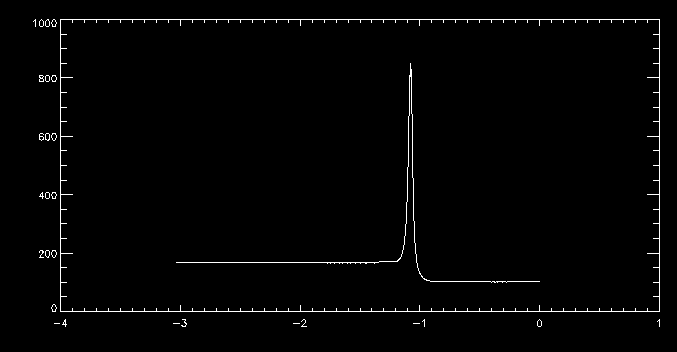
The first is just a graph of the tube in the x-z-plane. The second gives the density as a function of x. Note the spike in the middle where the two flux tubes meet, and that the density is lower on the right, in the vertical section, than it is on the left.
Continuing from last week, this week I have been doing a parametric analysis. Based on the code written last week, my goal has been to find how the maximum velocity and momentum trend with changing angle and density. The following contour plot gives a good idea of how they behave:
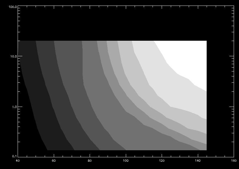
This gives the maximum of the z-component of velocity as a function of the angle between the lower tube section and the negative z axis, and of the log of the ratio of the densities (lower tube over vertical tube). The primary difficulty in this work was the sheer number of times the code had to be run to give an idea how it behaved. Now that that has been done, further analysis is relatively easy.
One valuable way I found to visualize these results was to make a graph of position with arrows indicating the velocity at each point, as can be seen here.
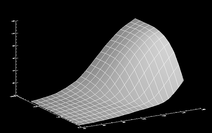
Similarly, I analyzed the maximum temperature and pressure achieved. This proved more difficult, as the code does not use a fixed time step. This meant that the data at high ratios and angles (the upper right portion of the graph) was simulating a far shorter period of time than than the rest. As temperature is expected to increase with time, this had to be compensated for. Despite this, those values tended to have much higher temperatures, even in less time, as the following graph indicates.
This week I have two tasks—first to figure out the cause of the aberrant behavior of my data from last week. To compensate for the decreasing time step and get a better idea of the temperature, I ran some simulations for many more cycles. Beyond a certain frame, however, these simulations simply return the dreaded value -NaN, for all variables. I suspect the x-resolution is too high, and so the differential length term in the calculations is becoming too small, causing division by zero.
The second task is to work on an analytic solution of the differential equations governing these flux tubes. Dr. Longcope has given me some code that gives us a start, but it currently is not particularly accurate, particularly when it comes to the temperature and pressure variables.
An abbreviated work week due to Independence Day. Little new research was done, as everyone is preparing for the SPD conference next week. My poster can be seen here (PDF, 1.5MB).
We've been mostly occupied with the conference again this week. I attended a number of the presentations. Tibor Torok's Harvey Prize lecture on modeling solar eruptions was especially interesting and relevant.
The -Nan problem from several weeks ago is still under investigation. In particular, large spikes form, usually consisting of just one point that deviates wildly from the rest of the data. We suspect this is a result of the Alfven speed becoming too great, causing the simulation to move information too quickly across the grid, essentially skipping data points. To test this, I took the run at 85 degrees and a 5:1 ratio, and have been testing at different magnetic field strengths (the Alfven speed is proportional to magnetic field). Up to B=100 gauss the problem seems not to occur, but above that it does, and the higher the field strength, the more quickly (in terms of time, not necessarily time steps in the simulation). Comparing the different runs at points in time where they should have progressed about the same amount, the error is again only present in those with high magnetic field.
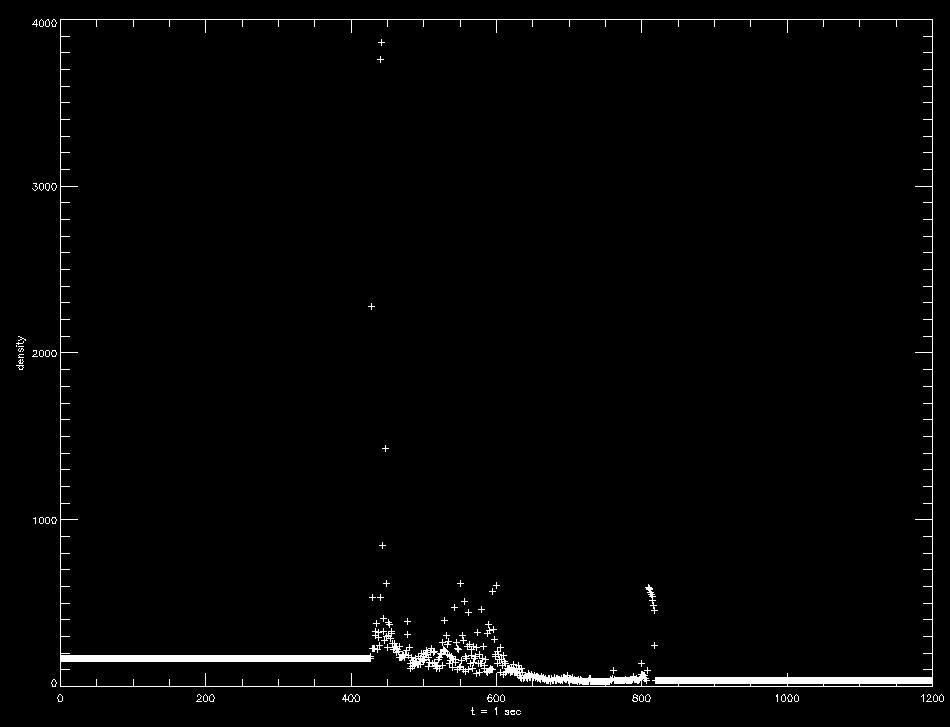

The upper image shows the density at 0.1 seconds with a magnetic field of 300 Gauss; the lower shows the same at 0.3 seconds with a magnetic field of 100 Gauss. The former is clearly less well-behaved than the latter.
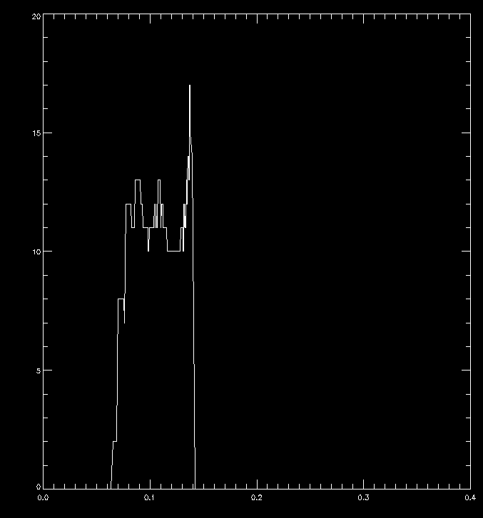
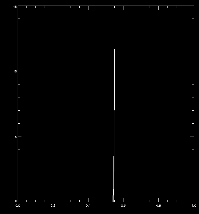
These plot the number of outlying data points over time, the first at b = 250 Gauss, the second at 150 gauss. At 50 Gauss, there are no outliers. Note that the apparent decrease in outliers toward the right is actually due to all the data being undefined.
All the runs to this point have been done with a fixed temperature difference between the ends of the tubes, specifically 5:1, with the vertical section being hotter. I am now working on modifying the code such that the pressure ratio is held fixed, and the temperature can then vary depending upon the angle and density ratio.
Update on part two from last week: the answer is, not much happens. The solutions are exactly the same as before.
Part one, however, turned out to be more interesting than expected. We noted that the curvature vector was becoming unruly when the spikes appeared. First we tried to simply smooth that out in the numerics, but that only exasperated the issue. The true cause, it turns out, is not in fact an error in the simulation, but a limit in the equations the code is solving. The equations of thin flux tubes assume a β value significantly less than 1. (β can be thought of as a way to see if tension or pressure forces predominate. At β = 2 they are equal, below that tension is dominant, shortening the flux tube. Above pressure dominates, elongating the tube, see here for more information.) It turns out that in the middle of the reconnection region, β becomes greater to large for the equations to hold. Increasing the magnetic field strength causes this to happen sooner, as does increasing the angle between tubes. Since we cannot get around this easily, it appears to be a condition we will just have to be careful to avoid running into.
Mostly finished with actual research. I am now working on my final presentation. A (very) rough draft is available here (PDF, best viewed in Acrobat Reader because the animations do not seem to work correctly in other viewers). I will update this with the final version once it is complete. Edit: this has been updated to the final version.