
|
|
|
||||
I will be looking at coronal holes in the Atmospheric Imaging Assembly (AIA) data from the Solar Dynamics Observatory (SDO) mission, as well as the Solar TErrestrial RElations Observatory (STEREO) mission Extreme UltraViolet Imager (EUVI) data, and use IDL routines to complete an analysis.
I have successfully made a webpage today. Now I can give daily updates on my research!
So, daily updates might have been a little optimistic. In this entry I'd like to cover my progress over this past week and present some of my creations. My tasks for this week were:
fov2carr.pro
First things first, I made this wicked movie Monday morning of 193Å AIA data from 28 May 2011 to 31 May 2011 in COLOR. You can watch it here. I know I need to work on my hyperlink skills, but you got a good look? Did you notice that it seemed to be 'blinking'? That was because not all of the frames had equal exposure duration. It is necessary that we find a way to 'normalize' the data.
Now after grabbing the AIA and STEREO data it had to be processed, as outlined above in tasks. First, I spent some time writing a code that would take the STEREO timestamps and rotate the frame to the nearest AIA date. The AIA data I acquired for the time range came on every hour, on the hour, and the STEREO data I acquired came every hour, thirty seconds after the hour. So currently my code simply takes the day and the hour from the STEREO timestamp and generates a new time stamp to match that of the AIA. Then I used drot_map.pro to rotate the image by that thirty seconds. I will go through an example with a frame from STEREO A to illustrate! Below is a map_plot of the original data
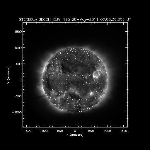
Now the next step was to adjust for the true longitudes. The AIA data holds the longitude of the center of the disk in stored in the map_aia.l0 part of the structure called say, map_aia. This is always called zero (Earth). The STEREO longitudes of the center of the disk, also stored in map_sa.l0 part of the structure called map_sa, are then with respect to the zero (Earth position). You can see this on the STEREO site, where is STEREO? in a nice diagram.
So, I wrote a code that would take the timestamps from each one of the three data sets and would input the year, month, day, and hour into sun.pro. If called, this programs returns the longitudes and latitudes of the center of the disk. For example, if I typed in the values for the STEREO A fram above, if I called lat0 and lon0, it would return to me:
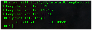
I then used those longitude values and added them to the longitude values found in the map structures already. I also needed to write a little check such that if the longitude (in degrees) was below zero or above 360° it would correct by adding or subtracting 360° respectively. These longitude values are very important because we would like to look at the STEREO A, STEREO B, and AIA data together on a Carrington projection.
With the adjustments the STEREO A data that we had before now looks like:

Not a large difference. This is because the image has only been rotated five minutes and some change, as you can see in the timestamp. The program drot_map.pro also cut off data not on the disk.
So that was the end of phase one. The data has been processed and now I want to feed it into a program that will detect the coronal holes (CHs). In the paper by Larisza D. Krista and Peter T. Gallagher a sophisticated method is outlined. For now, I will use "cheap" thresholding to find the CHs. I call my first stab at this cheap_detect.pro. In this program I "normalize" the data over duration of exposure by finding the mean value of each frame where it is not equal to zero and then dividing the data by that value. Then, if the map is rotated, I unroll it with rot_map.pro. This is necessary for the STEREO data.
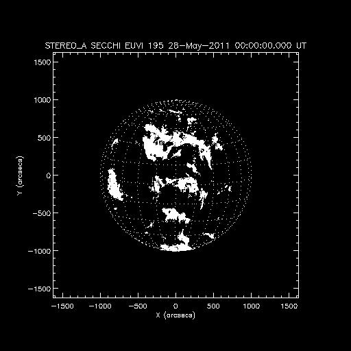
Next I make a mask to cover regions not dimmed, eliminating data outside the solar disk and at every value and I impose the thresholing criteria to create a byte map. So, I create a map structure where any value les than 0.8 is a 1 and any value greater is a 0. This is how I detect the CHs. I simply adjusted the 0.8 value until I was satisfied it picked out the CHs. A plot of the resulting map structure can be found below for my STEREO A frame example:
The next stage is to feed this into a routine that with turn it into a carrington project! I used Chris Lowder's fove2carr.pro. The result:
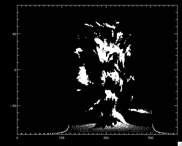
Fig. 1. Output of the fove2carr.pro from May 28, 2011 00:00 UT. Carrington projection of detected coronal holes. |
The goal was to project all three instrument's data onto one carrington project and in that way get a view of nearly the entire sun. With such a project over a period of time, say 28 May 2011 to 31 May 2011, we could watch the dim reagions evolve! A view of the AIA, STEREO_A, and STEREO_B data displayed together on a carrington projection can be seen below:
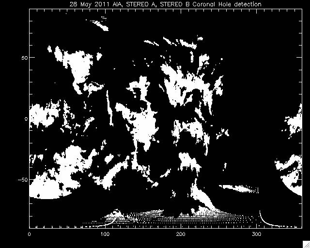
The regions at the bottom and top are not altogether trustworthy. Larisza D. Krista and Peter T. Gallagher in their paper suggest discarding the data above 60° and below -60°. So the projection would look more like this:
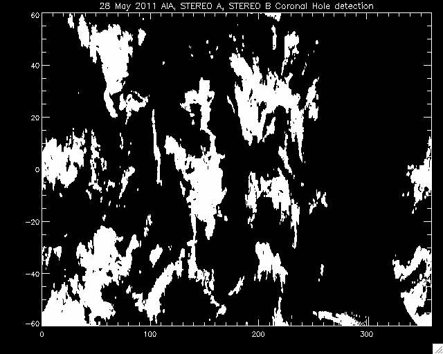
Now, with a more sophisticated thresholding technique we can more accurately detect the CHs and observe their evolution. The current goal is to write a program that can, given a start date and end date:
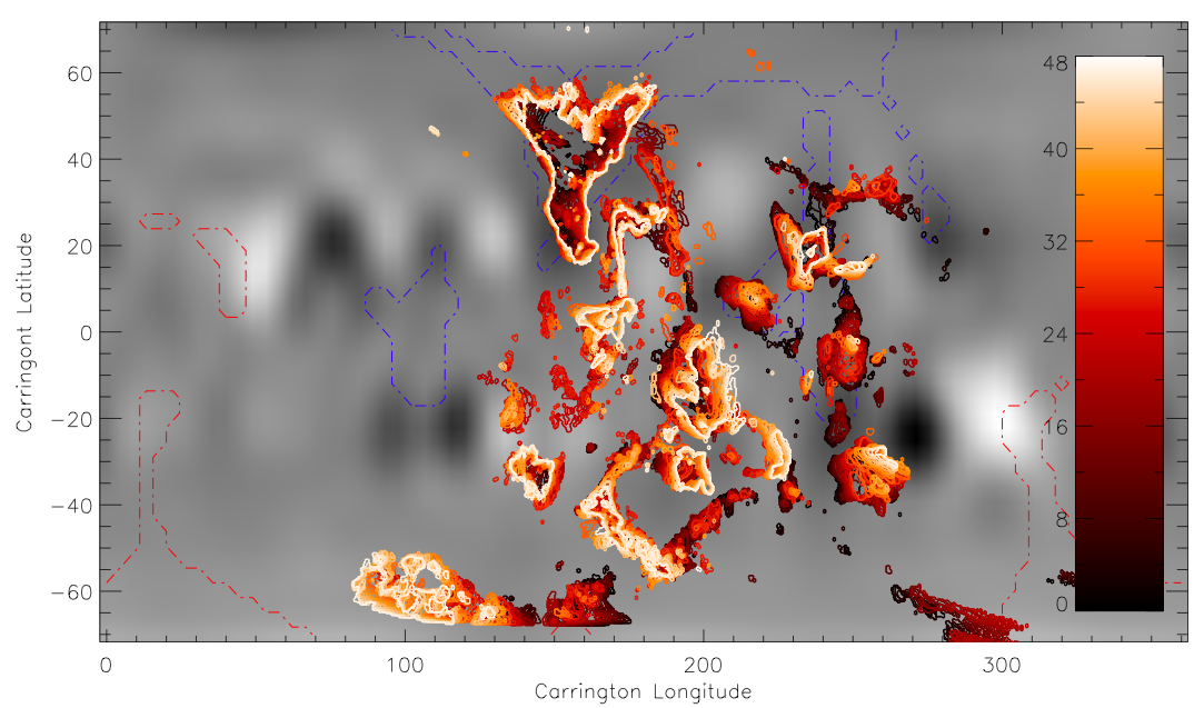
Finally, a nice plot of the latest results of the code(s) can be found below:
This week I have been working on a piece of the proposed coronal hole (CH) tracking routine and it is coming along quite nicely. My code, ch_threshold.pro, calculates threshold values for each frame of AIA, STEREO A/B data. To do this the code breaks each image of the sun into sub-regions (four seems to work well at present) and generates a histogram of all the values in that sub-region. It also calculates the quiet sun value of the region and searches for the local minimum in the histogram between 30% and 70% the quiet sun value. This minimum value that acts as the threshold value below which are (hopefully) the holes and above the rest of the data.
Below are some results of the CH detection with the original image divided into four subregions, and the mean value of the threshold values applied as the threshold value for the entire frame.

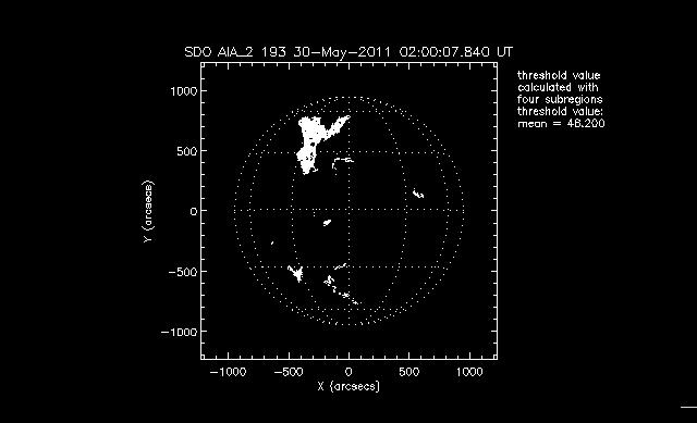
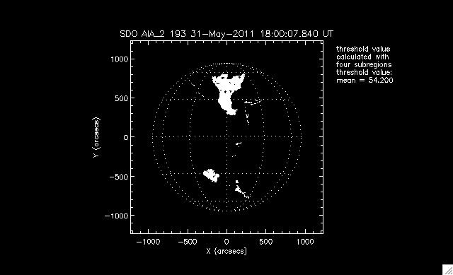
Now dividing the image up into nine sub-regions, I wasn't as impressed by the CH detection. The code seemd to pick up a lot of other areas that we're not interested in. When these were all averaged the threshold value appeared too high:
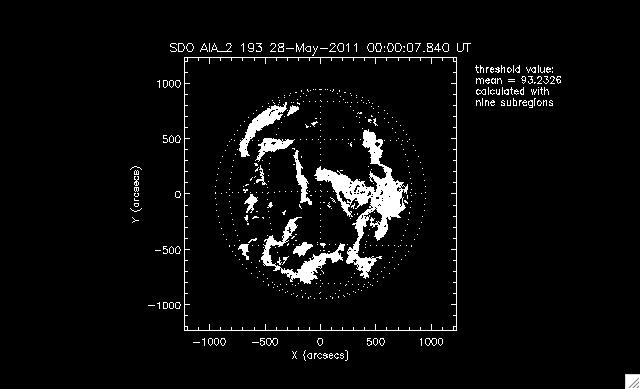
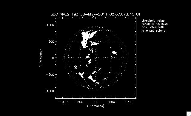
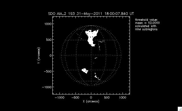
Evidently larger subregions are more effective at generating a good mean threshold value to detect coronal holes. These images above give you a rough idea of what I am looking at currently. We have yet to apply smoothing techniques in any of these, which will be a necessary step in the future.
So ch_threshold.pro appears to be up and running and is now integrated into ch_track.pro, our coronal hole detection routine. There are a few minor kinks yet to work out that Chris will be plugging away at in the next day or so. The next step for me is to begin using the Helioseismic and Magnetic Imager (HMI) data to look at the magentic field of the sun. Once the coronal holes are detected by ch_track.pro, we can use those coordinates and the HMI data to calculate the total magnetic flux through the region. Being able to calculate this flux will enable us to identify the dominating polarity of the coronal holes. It will also allow us to distinguish between coronal holes and filaments!
I gave a brief (roughly 20 minute) presentation to the solar physics REU group and mentors last friday. In this presentation I gave a brief overview of coronal dimmings and their relation to CMEs as well as described our strategy for detecting the coronal holes. Some information from the talk:
What are coronal dimmings?
Coronal dimmings and coronal mass ejections
Automated detection
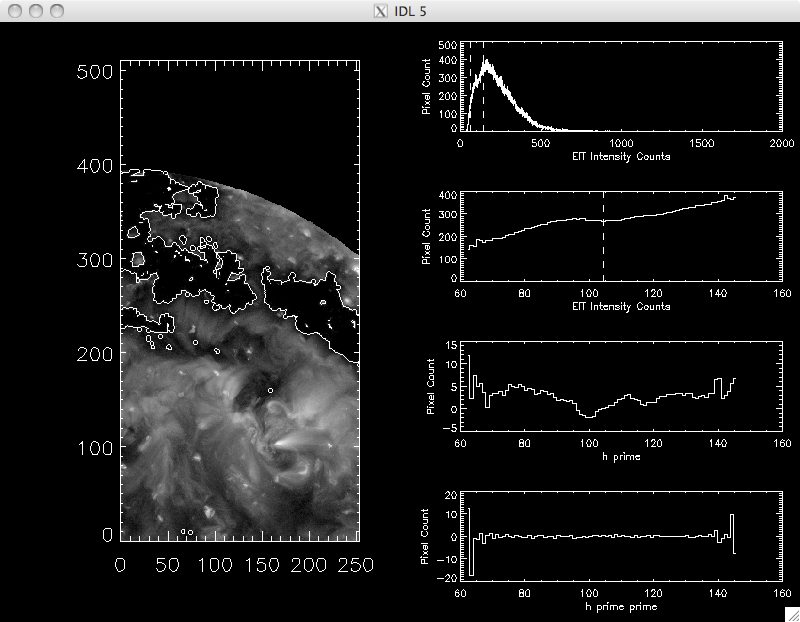
Here is an image of a successful attempt by ch_threshold.pro to pick out a thresholding value:
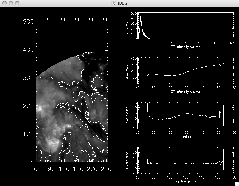
and an unsucessful attempt:
Looking to the future, once ch_track.pro is fully functional, we'll want to run it through it's paces, testing the code on several data sets that include both active and quiet periods of time. Basically, we'd like to try and trick the code so that we can correct for any ways it may get "stuck." With those data sets we'd like to take a look at charcteristics such as
pfss_viewer.pro, a program I can run through IDL, which allows me to look at the magnetic field lines extrapolated from the HMI magnetograms. I will also busy myself finding data sets challenging enough to be worthy of the greatness that is ch_track.pro and reading more on coronal holes from every solar REU student's favorite book: the Encyclopedia of the Sun.
And example output of the pfss_viewer.pro can be found below in Fig. 2:
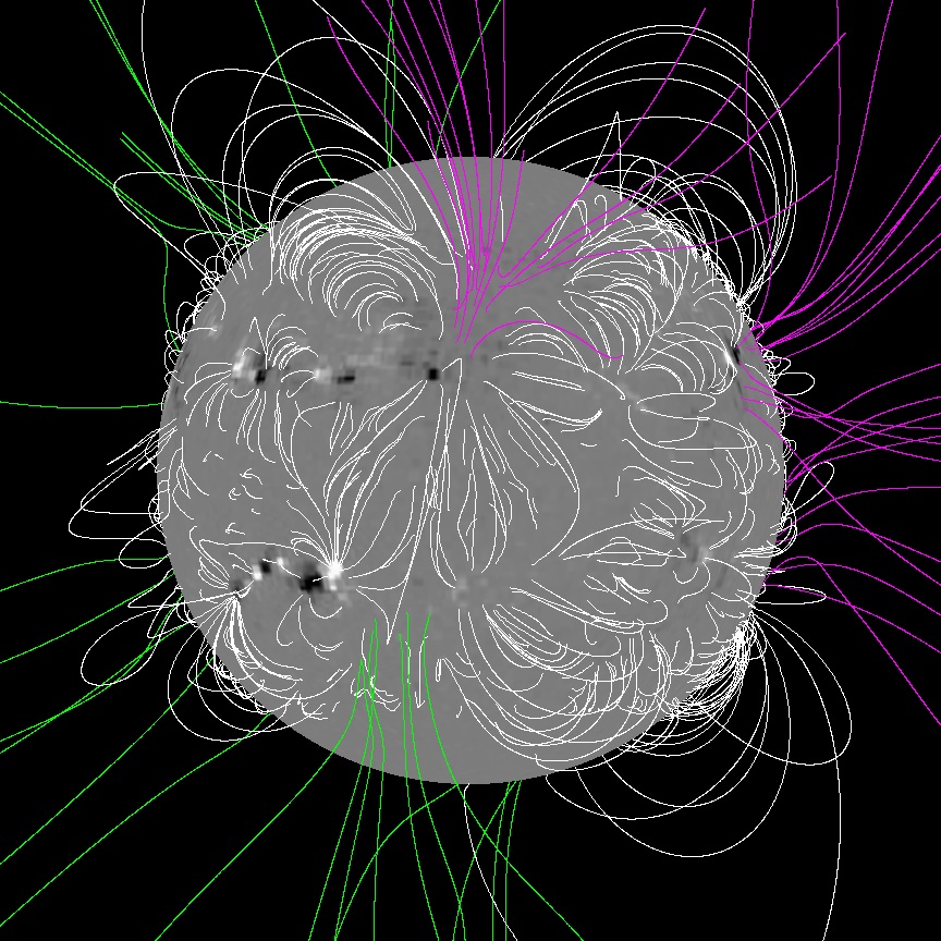
Fig. 2. Output of the pfss_viewer.pro from May 31, 2011 18:00 UT. Open magentic fields lines are those in magenta and green, closed in white. |
Compare this to the May 31, 2001 18:00 UT image in the June 16 entry above. You can see the open magentic fields lines, those in magenta, are going into the large coronal hole on the northern hemisphere of the sun. While we're on the subject, the green magentic field lines are coming out of the sun and the white magentic field lines signify closed loops.
In unprecedented fashion, I am writing for a second consecutive day! This morning I worked on the source code of this page. In order to publish anything at the beginning of the summer, I copied a past REU student's page. Unfortunately it was quite messy. In the process of cleaning it up, I've learned much html and I hope that this will encourage me to be more active in my web logging.
I've been working my way through several articles that Chris recommended in order to learn more about coronal holes, coronal dimmings, and detection methods. I would like to keep a citations page of sorts throughout the summer for future use and the interest of any reader, if I actually get one. I am thinking that I will make it a link on my Navigation bar.
And I did put it on the Navigation bar! Go ahead, click on it and check it out.
So some questions I would like to answer are: Why study coronal dimmings? What information do we get from them? What makes looking at them challenging or easy? Where do we see a study like this going?
Recently we've been struggling with acquring a few data sets to run through ch_track.pro, but Chris has data from the last three months at twelve hour cadence prepped and I have one day, March 19, 2011 7UT thorugh March 20, 2011 8UT at one hour cadence ready to go as well. Hopefully the two (a detailed shorter data set and a less frequent sampling over a long period) will allow us to fully test the capabilities of ch_track.pro and begin moving forward with the project.
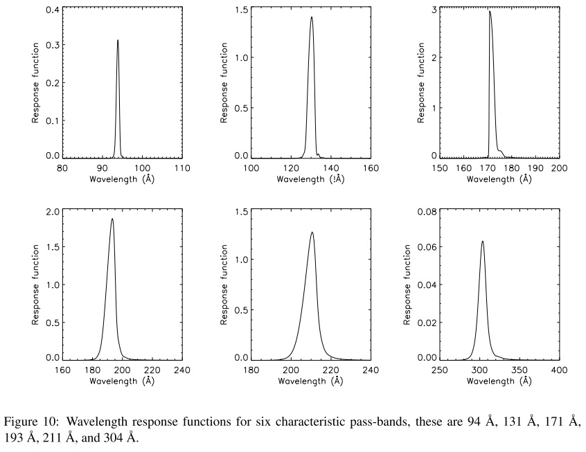
I am also keeping up on my reading and was first introduced to the concept of a resonse function in Brown, Marsh, and Bewsher's article on working with SDO data released at the beginning of this year. A response function is an equation that describes the reaction of a system, in our case a telescope, to a stress/stimulus, in our case electromagnetic radiation. So, it is like a translation between counts one gets from a .fits file and an actually meaningful quantity such as temperature and wavelength. For each broad band filter on the AIA telescope there are response functions that will center at the wavelength and temperature thought to be observed. Below are plots of the wavelength response functions for the AIA telescope:
And the temperature response functions:
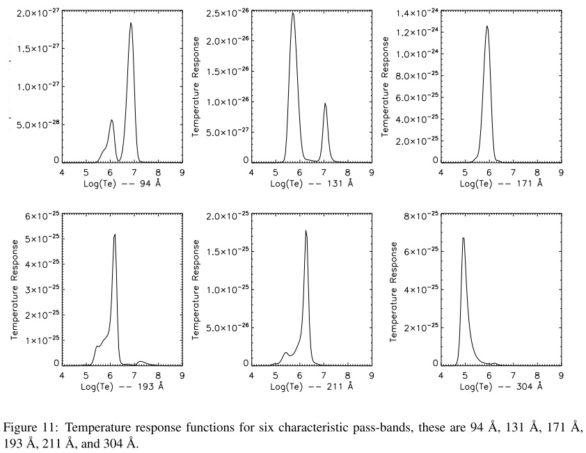
Unfortunately, the response functions of an instrument such as those on SDO takes some time to perfect and as the SDO mission is yet young, the response functions available for AIA are not completely trusted. But it is the job of another scientist to work on these response functions and in the meantime we may use what is provided and wait patiently.
With only four weeks left in the REU program its time to take a look at current and long term goals of the project.
get_hc.pro and open_reg.pro
In Fig. 3 I have a nifty flow chart representing what we're doing with the suite of programs written this summer and the PFSS codes already written.
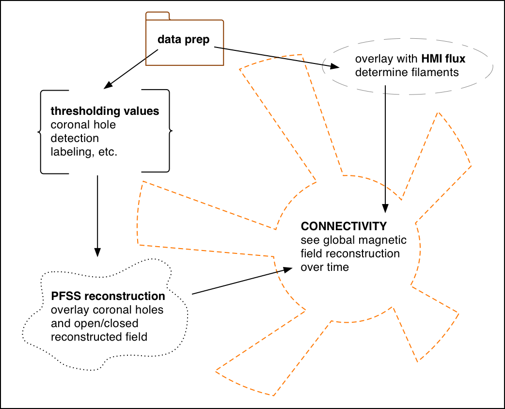
| Fig. 3. Flow chart of (conceptually) where we're headed with the written codes. |
So now I have STEREO/EUVI, SDO/AIA, and HMI data for March 19, 2011 7UT thorugh March 20, 2011 8UT. I ran this data through secchi_prep and aia_prep respectively and have a save file ready to go. (Note: I also had to check manually that there were no corrupted frames--there were--and replace them with the nearest uncorrupted frame.) That out of the way, I wanted to generate the PFSS reconstruction of the magnetic field using the Wilcox Solar Observatory (WSO) harmonic coffecitents. WSO, located just west Standford University, is a ground-based observatory that looks at the global magentic field of the sun. Available WSO data includes magnetograms, synoptic charts, coronal fields, and harmonic coefficients. The harmoic coeffients are what I want. These are found by modeling the magnetic field based on conditions in the photosphere, then deconstructing the field. Here's what the WSO site has to say on the matter:
The tables of harmonic coefficients we use are found using radial photospheric field boundary conditions and can be requested from this site. Using these harmonic coefficients and the codesThe field in the corona can not be measured directly. However the field can be modeled because it's basic structure is determined by the conditions in the photosphere. We use a potential field model to compute the field about 1.5 solar radii above the Sun's surface. That's the height at which the field pattern becomes fixed. That pattern is carried out into interplanetary space by the solar wind. It takes about 4 days for the pattern to reach the Earth. The model isn't very good at predicting dynamic changes in the corona.
The "los" (line-of-sight) method has been used and published for many years; that model assumes that the field measured in the photosphere may be nonradial.
The "rad" (radial) method is probably better. It assumes that the photospheric field is radial in the photosphere. The best source surface radius is 3.25 rather 2.5 solar radii for the los model.
...
The photospheric and coronal field can be decomposed into spherical harmonics. The monopole, dipole, quadrupole, etc. components can be used to reconstruct the field at any height between the photosphere and source surface. There are no plots, but you can get the coefficients in tables. The harmonics computed using the two models described above are slightly different.
get_hc.pro and open_reg.pro I was able to make a high resolution carrington project of the global magentic field. The code took roughly 3 hours to run! The red dashed lines trace the regions of positive open field, the blue of negative open field. See below in Fig. 4.
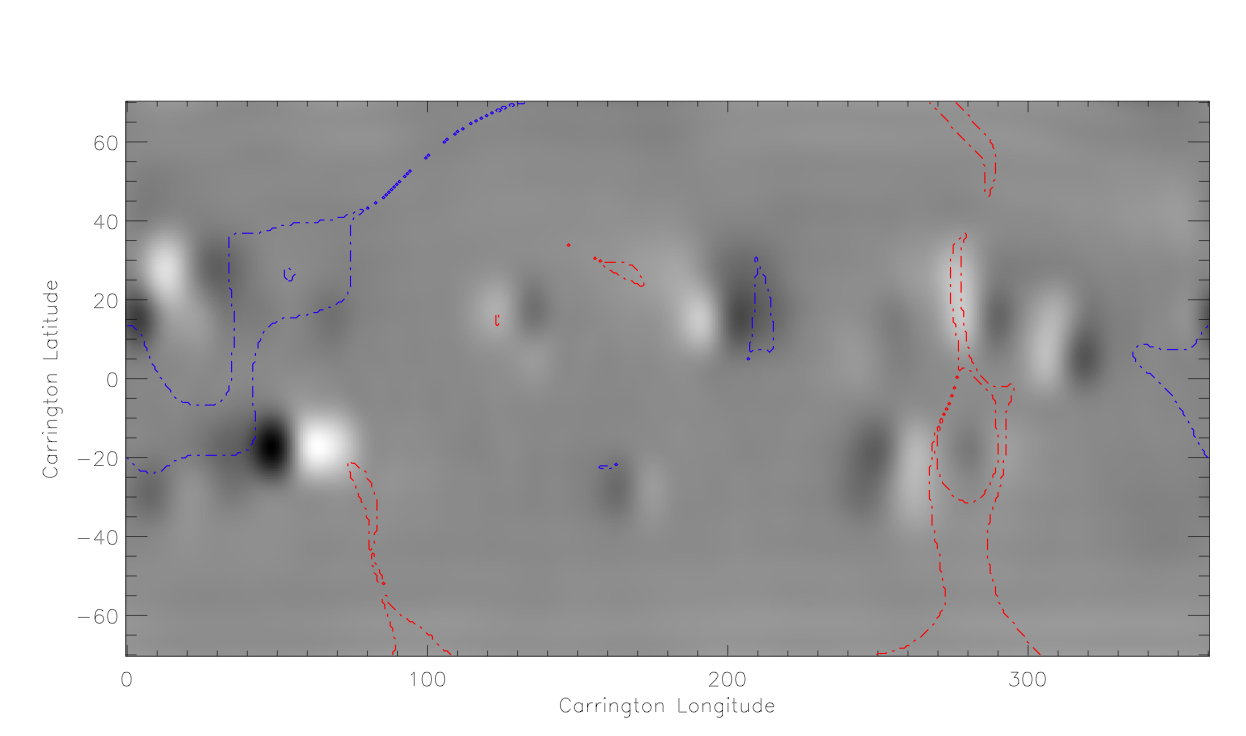
| Fig. 4. Carrington projection of magnetic field centered on March 19, 2011 7UT, reconstructed from radial model using WSO harmoic coefficients. Red dashed lines trace the regions of positive open field, the blue of negative open field. |
Next, I want to take a look at the field a little before through a little after in the field of view (fov) frame.
As it turns out the magnetic field of March 19, 2011, the date I selected more or less at random, is quite intesting. This can be seen especially in the fov PFSS reconstructions in the short term study from my July 8 entry. On Solar Monitor I took a look at the x-rays around that time and just after the date range I have analyzed there are a few flares on the 21st, 23rd, and 24th of March, as you can see below in the site's output:
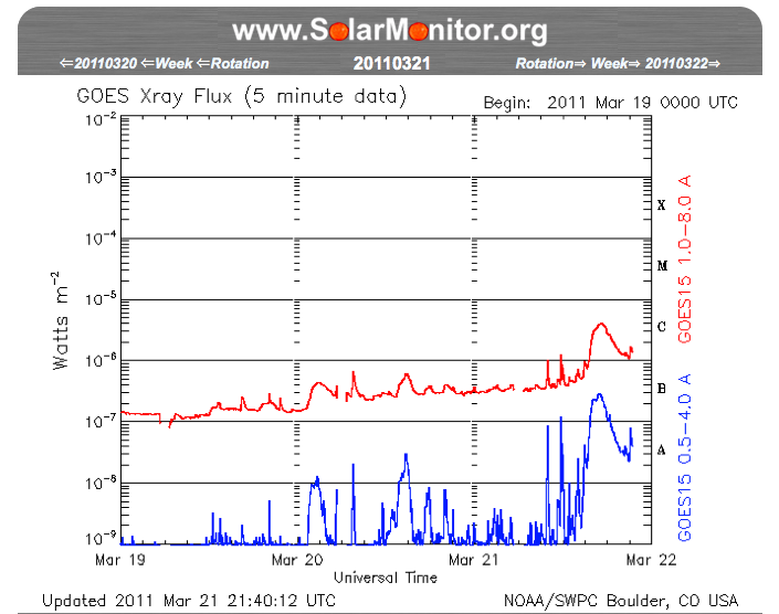
| Fig. 13. Solar Monitor x-ray data from GOES from March 19 - 22. |
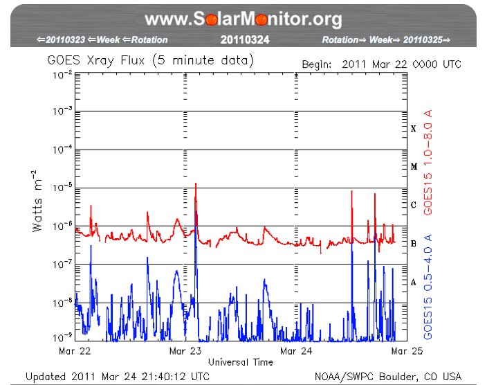
| Fig. 14. Solar Monitor x-ray data from GOES from March 22 - 25. |
The largest flare on the 23rd of March actually appears to reach X-class. So, we decided to extend this particular survey to the 25th to get a better look at a magnetic field over a period of time with several active moments/regions. I download the corresponding SDO/AIA, STEROE/EUVI, and SDO/HMI data. Then I proceeded to prep the data and run it through ch_track.pro.
As it turns our there are several hours of data missing form the STEREO_A data, so in to keep the data sets equal length I removed the coressponding files from SDO/AIA and STEREO_B/EUVI. The missing hours were 2011/03/22 07 UT - 2011/03/22 15 UT. Now I would like to run this data through ch_track.pro as I did with the data sets from my July 8 entry.
Further, we have introduced a new section into ch_track.pro that will get data on the coronal hole map produced by the program. We wanted to be able to label all of the detected coronal holes and be able to track them over the date range of the data set. This was done with total.pro and label.pro, imposing the label map onto the chmap retroactively. Then, as we track them we can calculate the area and centroid over time. At the moment there are too many detected CHs--we've yet to impose a size threshold--so I cannot generate a movie that would illustrate what we've done, but that is soon to come!
Also, while we're on the subject of things to do, ideally by the end of the summer we'll have three data sets: (1) long term low cadence, (2) shorter term medium cadence, and (3) very short high cadence. The March data will work at the Medium cadence, the April - June 2011 data as the longer term study, and we have yet to acquire a very short, high cadence set.
Below I've posted a link to the Medium cadence page. I think at some point I will want to move these pages to the Final Reearch page, but for right now this will do:
So what have been up to lately? I've been aquiring another medium cadence (1 hour) data set from June 7, 2011. There was a nice M-class flare that day, and for once it appears I will be able to get a full data set (no missing hours). Getting all four instruments (SDO/AIA, STEREO_A/EUVI, STEREO_B/EUVI, and SDO/HMI) to provide good data for the same time range is turning out to be quite a challenge.
Our code, ch_track.pro now has a few lines that will allow us to track the area and centroid of each CH detected by ch_track.pro and labeled by label.pro. I am hoping to generate a few plots to check out the preliminary results on a complete data set such as the March 19, 2011 data. We're still on track to have 3-4 data sets run through the code, tracking the CHs and then taking a look at there comparison with the PFSS reconstructions.
Besides running the data through our code(s) and generating the corresponding PFSS reconstructions, I would like to spend a good amount of time reviewing what exactly we are doing when we generate the PFSS reconstructions. I understand on a very simple level, but it is one of our primary ways of chekcing out the magnetic field lines coming out and going into the sun. There are some pretty intense assumptions going on there that I'd like to bring up, maybe leading to motivation for more and better models of the sun's magnetic field in the corona.
We can compare the CH map output of July 21, 2011
ch_track.pro and the PFSS reconstructions, displayed at Carrington projections, in a couple of ways:
We can also note the polarity of the open-field regions (the CHs) in the PFSS reconstruction. Further, using SDO mission data we can look at the following from the AIA CH map and the HMI magnetograms:
Recall the total flux through the detected CH can tell us whether it is indeed dominated by a single polarity and is thus a CH or if there not significantly more positive or negative flux, indicating a likely filament.
Because we do not have an instrument on STEREO that measures the line-of-sight magnetic field, we cannot look at the flux through the CHs once they've left the view of SDO/AIA. It is nonetheless useful to observe this flux while we are able.
In time we would like to be able to take the Carrington CH map, the final output of ch_track.pro, and convert that back to a FOV projection so that we can overlay it with the SDO/HMI map structure and obtain the flux. At present this is not how we are doing it, rather we are taking the SDO/AIA CH map only, before Carringotn projecting it, and overlaying that with the HMI FOV map structure. This is the simpler way to do it, but there is one downside---now the FOV CH map labels do not match the Carrington CH map labels. The labels are applied later in the code to the Carrington CH map. This is something we hope to address soon. In the meantime I can viusally confirm that one or two CHs are the same CH, even as they will be labeled differently, and study them individually.
ch_track.pro is capable of producing at the moment.
It is the beginning of week 9 of the Solar Physics REU program here at Montana State university and really, the beginning of the end. It is now time to start generating my final results and begin drawing up my presentation. My goals before the end of the summer are as follows:
ch_track.pro, tracking a few CHs and filaments across the solar disk during this July 2011
ch_track.pro to complete analysis of each, including plots of CH area over time, centroid, contour boundary evolution maps, and all those of the type presented previously here and here.
Thus, before I present to the Solar physics group here, I should have several plots for each of the data sets that will allow us to look at CHs in SDO/AIA, STEREO_A/EUVI, STEREO_B/EUVI, and SDO/HMI data. We should be able to observe charactersitics of these detected CHs such as area, centroid, position over time, persistance, corresponding threshold & quietsun values, corresponding PFSS reconstructions, and total flux.
I shall begin dowloading the data immediately and integrate the lines from Well, I've completed the first goal mentioned in the above July 25 entry and have a prepped data set from July 11 through July 20, tracking a lovely CH and filament. I have run the data set through When I arrive at the stage where I total the SDO/AIA fov coronal hole maps (chmaps) in order to label them, I notice that the CH and filament that I know to be there have joined to become a giant blob. There appear to be roational effects in the totaled AIA fov chmap, as seen below. I cannot look at the flux through the CH and the filament if the mask looks like this! Notice that, if I were to rotate a frame when the CH and filament are closer to the center of the disk, both are distinct and where I would expect them to be. But if I were to rotate a frame to the same date when the CH and filament are nearer the limb, the rotated fov chmap does not appear to be where I would expect. Thus, totaling several such rotated maps, I produce a rather messing chmap mask which, when labeled, does not allow me to look at the CH and filament flux separately. This in turn does not allow me to characterize the flux with I was, however, able to take another look at the histograms I made for last weeks presentation, found here, and rebin the HMI flux data. New plots of the histograms can be found below. I then ran the rebinned data through I have a clue as to why totalling the fov AIA chmap is giving me nonesense: see this video of the frame by frame representations of my 'rotated' images. So clearly I need to figure out why my structure tags are not all agreeing with each other. I thought I had updated the x-center and y-center, but there is something wrong nonetheless. So it's my last day in Bozeman, MT and I will be very sad to leave the mountains and minds I have encountered here behind me. I leave bright and early tomorrow morning (4 AM) for a long, arduous jounrey back--though it will be nothing like that of my St. Andrew's colleagues, or Rahul headed back to India. I have posted a copy of my final presentation on my final research page if you woudl like to check it out. The presentations occued this week and went very well for all involved. I wish to thank Chris Lowder, Jiong Qiu, and the entire Solar Physics group at MSU once more for an amazing and inspiring summer. This has really given me a chance to see what a life of reasearch could offer and I look forward to applying to graduate programs in the fall. Thanks again everyone!ch_flux.pro (which overlayed the CH fov map and the HMI data) into ch_track.pro. Next I will run that data through this newest ch_track.pro and generate histrograms and skewness values such as those found in my week 8 presentation. It is our intention that this give us a typical skewness value for the flux of a CH, since for this data set we can visually detect the CHs (more dark or light patches in the magnetogram where there is a 'dim' region) quite well.
July 26, 2011
ch_track.pro and am in the process of overlaying output on top of coressponding SDO/HMI data to find total flux through detected CH(s) and filament, and to observe the statistics thereof. Unfortunately I've run into a slight hitch.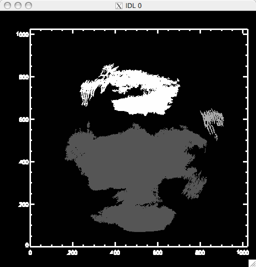
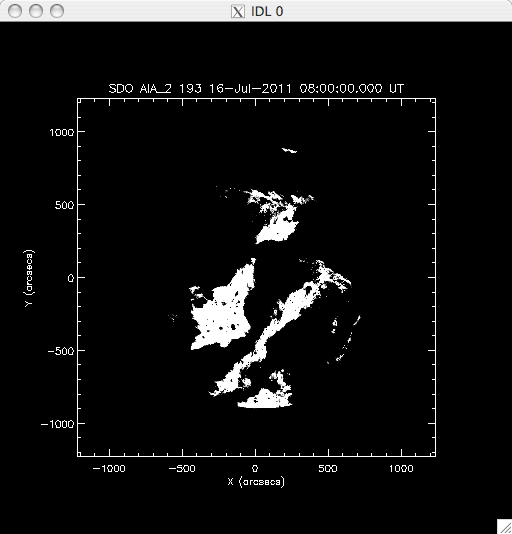
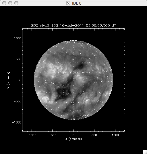
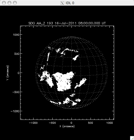
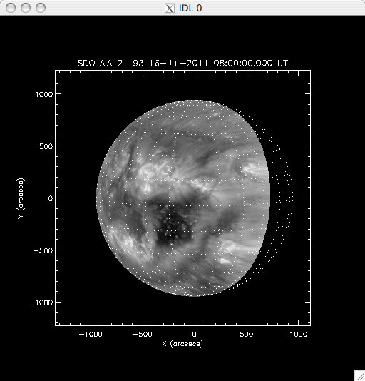
moment.pro to find the mean, skewness, variance, and kurtosis.
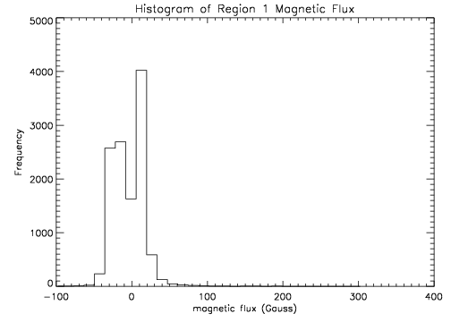
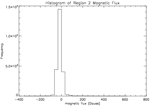
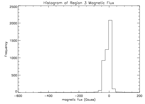
moment.pro, and found the values in the table below:
Output of
moment.pro
Region
Mean
Variance
Skewness
Kurtosis
Region 1
400.067
975983
2.42794
4.86886
Region 2
787.867
7787150
4.01734
16.3099
Region 3
149.000
209154
3.09970
8.98840
2:30pm
August 5, 2011