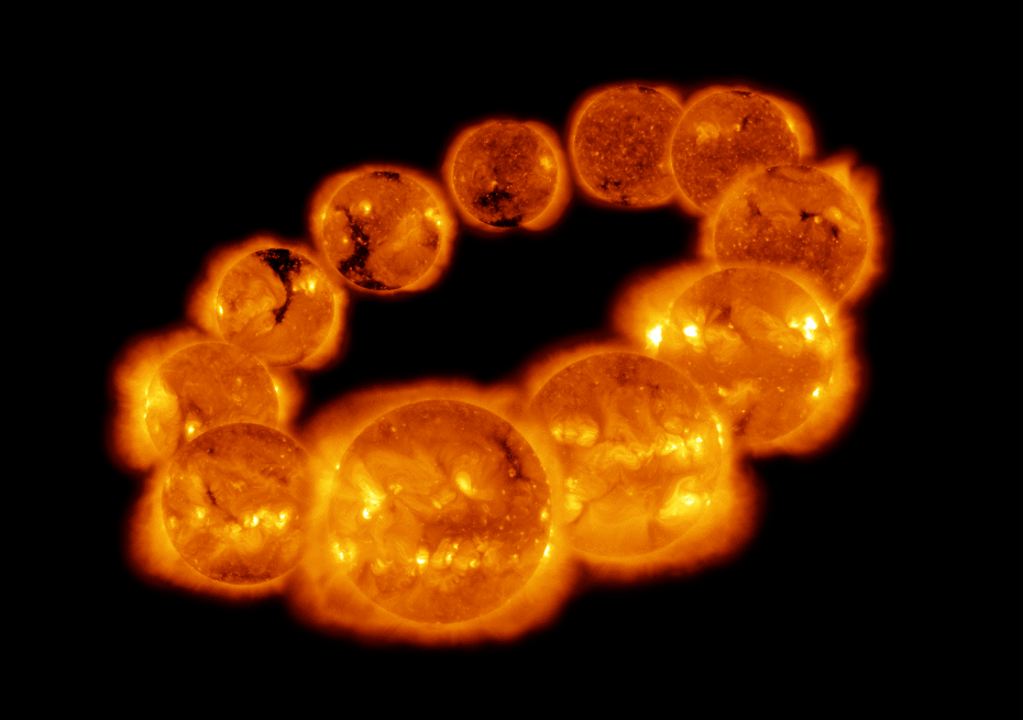
Solar Soft X-ray Irradiance with Hinode/XRT
Shannon Boland (University of Wyoming) and Aki Takeda
as a MSU solar/space REU 2022 project.
Project descriptions
Montana State University (MSU) is home of Hinode/XRT Synoptic Composite Image
Archive ( SCIA ), which is the archive of soft X-ray full-Sun images obtained
with the X-Ray Telescope aboard the Hinode satellite. Our images are posted
daily to the SolarMonitor, a popular site for solar researchers to check the
current solar condition.
With this archive, we can study solar activities in terms of the Sun's radiation
in soft X-ray wavelengths. In this project, we will process the XRT/SCIA images
taken from 2006 to present to derive the soft X-ray irradiance during this period.
We will learn how to process Hinode/XRT FITS data for quantitative analysis using
the data analysis software IDL(Interactive Data Language): data selection,
derivation of temperature and emission measure, calculation of the XRT irradiance
in the physical unit (W/m^2), etc. This project is continued from 2021.
This year, we will put emphasis on the data calibration to correct characteristic
change of the instrument over 15 years of operation, and comparison with the
observations by other instruments measuring the solar cycle variation.
As a bonus, the student will have a few opportunities to watch and learn how
an international satellite project like Hinode is operated. As one of US
institutes participating the Hinode satellite operation, we have a duty week in
July, in which we take control of the XRT observation.
Weekly goals
- Week 1 (5/31 -- 6/3) :
- Get familiar with IDL (Bootcamp by C. Zhu on 6/1, 9am- @room#258)
- Read "Encyclopedia of the Sun" to study background of the project
(sections 8.4, 8.5.).
- Introduction to Hinode project and XRT instruments.
- Introduction to XRT data handling with IDL.
- read XRT level0 data (sample_read.pro)
- calibrate XRT data (sample_prep.pro)
- make a composite image(sample_comp.pro)
- Week 2 (6/6 -- 6/10) :
- Get to know about SCIA data.
- Understand the project goal and steps to get there.
- step 1: data selection
(find usable image pairs of thin_Be and Al_mesh)
- step 2: collect total intensity within 1.1 Rs.
- step 3: derive averaged temperature(Te) and Emisison Measure(EM)
for each pair.
- step 4: convert Te and EM to solar irradiance in the unit of W/m^2.
- Finished until Step 1 and Step 2.
- Preparation for the short presentation on Friday 2pm. (well done!)
- Week 3 (6/13 -- 6/17) :
- Learn about the Filter Ratio Method.
- Calculate Te and EM for the additional months (with Chianti ver.9).
- Calculate Te and EM with Chianti DB ver 10.0, assuming different
abundance sets, for the whole mission (great job!).
- Learn about how to make IDL procedures and run them in sequence.
- Week 4 (6/20 -- 6/24) :
- Make mission-long over plots showing different Chinanti versions
or different abundance asumption.
- Calculate Te and EM with a modified XRT effective area functions.
- Start working on the investigation of the "height dependence"
(SCIA data for 2021/10/16-17 might help).
- Preparation for the 2nd bi-weekly meeting on Friday 2pm (well done!).
- Week 5 (6/27 -- 7/1) :
- Process mission-long data with a modified XRT effective area functions.
- Advance "height dependence" project.
- Understand the method converting Te and EM to irradiance.
- Week 6 (7/6 -- 7/8) :
- Preparation of mid-term presentation (excellent!).
- Advance indelendent project (height depenence study).
- Week 7 (7/11 -- 7/15) :
- Start converting Te and EM to Irradiance in W/m^2
- Propose special observation to XRT to study high corona.
- Sneak peek Hinode operation meeting (7/13 19:30-)
- Advance independent project (find signal increase with radius).
- Week 8 (7/18 -- 7/22) : Concentrate to the independent project.
- Week 9 (7/25 -- 7/29) : Independent project + preparation of the final presentation
- Week 10 (8/1 -- 8/4) :
- Final presentation! Excellently done!
- Organizing/cleaning working directories.
- Prepare final document of the project (like abstract of the science meeting presentation).
Resources
just a memo for the 6/9 meeting
CCD detecter (Charge Coupled Device)
photoelectric effect
how CCD works
memo for the 6/13 meeting
memo for the 6/20 meeting
Chianti atomic database :
- an up-to-date atomic database and associated codes (IDL, Python),
- for the analysis of optically-thin line and continuum plasma emission (like solar corona).
- developed by a group of scientist from US(NRL) UK(Cambridge) and
Italy(Arceri Astrophysical Obs.
- version 1 released in 1997.
memo for the 6/30 meeting
X-ray radiation from coronal plasma
- free-free emission
- free-bound emission
- bound-bound emission
coronal emission mechanisms
sample X-ray spectrum
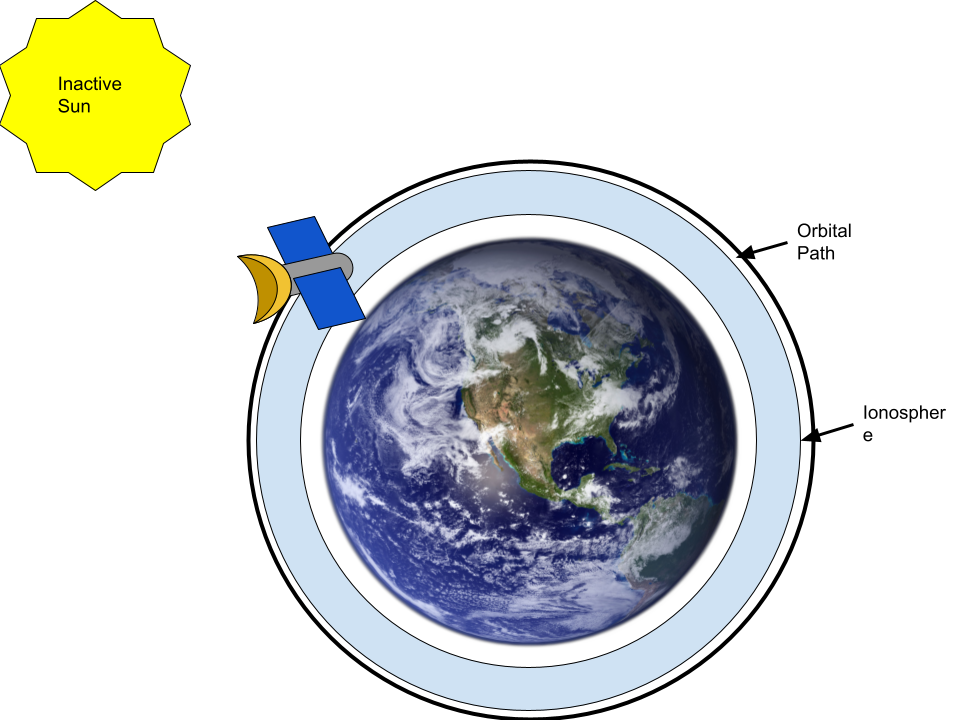
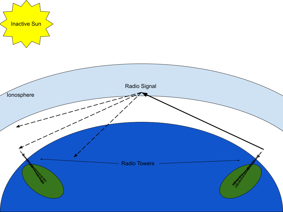
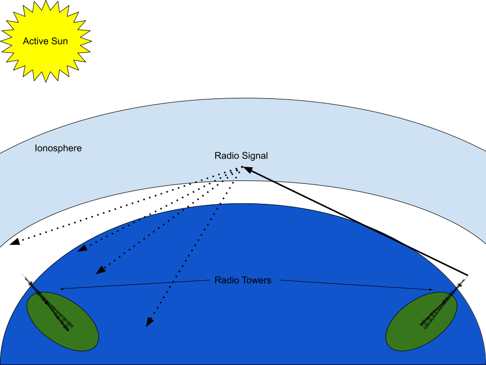
Solar X-ray radiation affecting to Earth
Google drawing by Shannon
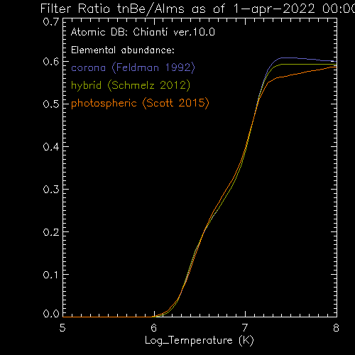
XRT response and filter ratio function corrected plots
[note: plots created by xrt_resp/get_fratio_amtb2.pro]
note for the 7/11 meeting
note for 7/12 meeting
Planning the special observation with XRT for this project.
- XOB#1CE4 was prepared (and modified).
- 0: dark images
- 1: Al_mesh synoptic set (2ms/125ms/707ms/707ms/707ms
/707ms)
- 2: Al_poly synoptic set (12ms/177ms/1.41s/1.41s/1.41s
/1.41s)
- 3: thin_Be synoptic set (16ms/500ms/3.78s/3.78s/3.78s
/3.78s/3.78s/3.78s)
- repeat 1-3 for 5 times. → 2 times
- duration: 10min 28sec → 8min 28sec
- memory: 435 Mbits → 237 Mbits
- pointing: (-411.0, 847.0) --- same as HOP344 the 10th pointing
[example: 2021/10/17 at 12:56UT ] ---.
→ (-530, 530)
--- similar to the post bakeout pointing #4 ---
- keep the pointing for 15 min before moving to the next obs.
This XOB (final form)
was scheduled to run on
2022/07/16 .
      Date & Time   Tracking  Offset-X Offset-Y */
         (UT)       Curve No.  (deg)    (deg)   */
2022/07/16 03:45:00    0     -00.1472  00.1472  /*  -530.0/  530.0 : # XRT high coronal structures. */
2022/07/16 04:00:00    0      00.0000  00.0000  /*     0.0/    0.0 : synoptic, shifted  23.5 min + HOP 349 */
The stray light image at the same pointing was also obtained on 2022/07/19
using
XOB#1CDC .
note for 7/15 meeting
- Comparison of different calibration parameters on thin_Be filters:
- no correction (except stray light subtraction from Al_mesh).
- filter contamination correction only on Al_mesh.
- filter contamination correction on Al_mesh and thin_Be (ver1).
- filter contamination correction on Al_mesh and thin_Be
(ver2: thin_Be thickness 2 times larger than ver.1).
It turned out that change of thin_Be thickness does not affect the result.
Will choose ver.1 as a representative value for thin_Be.
- Comparisons we will show in our final presentations:
- Chianti ver 9 and 10 with coronal abundance.
- Chianti ver 10 with different abundance sets
(corona, hybrid, and photospheric).
- With/without filter contamination correction
(with Chianti ver 10, coronal abd).
Comparare "step3" and "newcal2" data sets.
Examples of Abstract

Aki Takeda (Research Scientist, Dept. of Physics at MSU)
