Magnetic Field Extrapolation

This summer, we began to focus on the magnetic structure of the progenitor before it erupted as well as the overall global magnetic field, building tools along the way to help us understand what is going on. The most important tool we have developed so far has been a program that extrapolates the magnetic field of a region on the Sun.

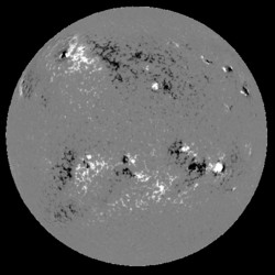
The program uses a line of sight magnetogram (like the one seen to the right) to determine the z-component of the magnetic field across the region. It then uses inverse Fourier transforms to determine the x-, y- and z-components of the magnetic field.

The program requires no inputs to run. Once called, it reads in a file that contains the dates, times and locations of all the magnetograms downloaded to date, prints that file on the screen and prompts the user to choose the magnetogram they would like to have loaded. If the user attempts to choose a file that is not on the list, they are notified of their error and asked to choose again. The appropriate fits file is then loaded and read into the program. This file is then converted into a map and run through a modified version of the IDL program sub_map.

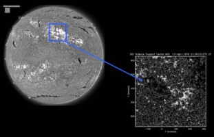
Sub_map plots the magnetogram and allows the user to select a subregion. The subregion is then converted to a 256 by 256 map centered on the middle of the location of the chosen area and outputted for further use.

It is necessary to make the outputted array a factor of 2^n so that it can be run through the magnetic field extrapolation program without anomalous outputs. The map of the selected sub-region, as seen to the left, is then plotted for the user to view. They are given the option to accept the region and continue with the program or to choose the area to be extrapolated again. Once a final region is selected, the data from that region is run through the magnet field extrapolation program.

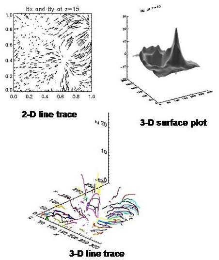
In the extrapolation program, data from the selected sub-region is run through inverse Fourier transforms to determine the x-, y- and z-components of the magnetic field. A 2-D image of the field lines and a 3-D surface plot of the magnetic field are produced. The program outputs three 3-D arrays, one for each component of the magnetic field. The user is again given the option to reselect the area of extrapolation or continue on with the program. Next, the components of the magnetic field are run through a line tracing program, which chooses a point at z=0 and interpolates the direction of the field line to the next point, until it has done so 2,500 times for each line. The user has the option to specify how many lines he wants to see, but the default is 50. The lines are then plotted in 3-D. The line tracing program outputs a cube holding the points that were connected by the trace, allowing the user to retrace the lines and view them at any angle. Finally, jpegs of all the images produced, along with a data file containing the information about the selected region and the extrapolated magnetic field components, are saved to the directory from which the original magnetogram came. The user is notified of the location of these files and the program is exited.

The program has three keywords, which allow the user to customize how it is used. The keyword "small" allows the user to select a 128 by 128 subregion from which the magnetic field will be extrapolated. This is useful for focusing in on smaller regions as well as helping the program to run faster. The keyword "directory" allows the user to specify the directory into which all of the files are saved rather than using the default. The keyword "nops" allows the user to prevent the program from saving any files at all. The optional outputs of the program include the infromation associated with the selected sub-region, components of the magnetic field and a data cube containing the lines connected by the line tracing program.

Now that we have created most of the tools necessary to analyze the magnetic fields of the progenitors, we want to see if there is any correlation between them and the direction of the magnetic field of a cloud when it reaches 1 AU. Currently there exist both large-scale and small-scale models that attempt to predict the leading field direction of magnetic clouds. Large-scale models function on the premise that eruptions are globally defined events whose orientations correlate with the solar dipole. Small-scale models, on the other hand, assume that only the local fields of the active region are what influence the leading field. However, neither of these models has been able to predict the leading field direction of magnetic clouds with accuracy much greater than that of flipping a coin. Thus, we have opted for an intermediate model in between these two extremes. We will be using a potential source surface model to describe the 3-D structure of the magnetic field in the corona which directly overlies the progenitor.