Numerical Simulation of Flaring Loops
Motivation
The post flare loops are comprised of a thermal and nonthermal
distribution of particles. Yet, few if any flare simulation codes
model both populations in tandem and allow them to ineract. In this
work, new simulation codes were developed in order to
model the thermal and nonthermal distributions and their
interactions in order to better simulate the emission signatures of
solar flares, and to provide a laboratory where theoretical particle
acceleration mechanisms can be tested against real observations.
Analytic
Loops
Below are simulated flaring loops. The geometry for the first
experiments were derived analytically using Green's solution for a
model post flare arcade with a current sheet. (N.B. This is
often called a Syrovatskii current sheet model in the literature. However,
the Syrovatskii solution is slightly different. See Bungey & Preist, 1995)
Geometry
Using the formalism developed by Bungey and Priest (1995), complex variable
notation is used to map the magnetic field lines associated with Green's
solution (Green, 1965) to a potential field configuration with a 2.5D current
sheet. A field line below the separatrix is chosen in order to avoid the
situation where B=0 along the field line which would cause a discontinuity in
the area of the loop. This is physically reasonable since a field line only
spends ~ 2 seconds in the current sheet (Fletcher & Martens, 1998) and it is
the evolution of the post flare loop that is our subject of interest.
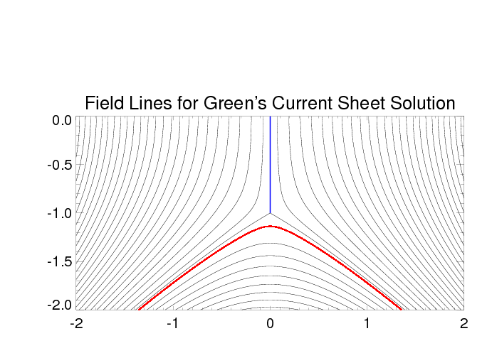
A contour plot of the magnetic field lines and current sheet generated by Green's
solution (Green, 1965). The field line we will use to describe our
loop is in red. The current sheet is drawn in blue and the units are arbitrary.

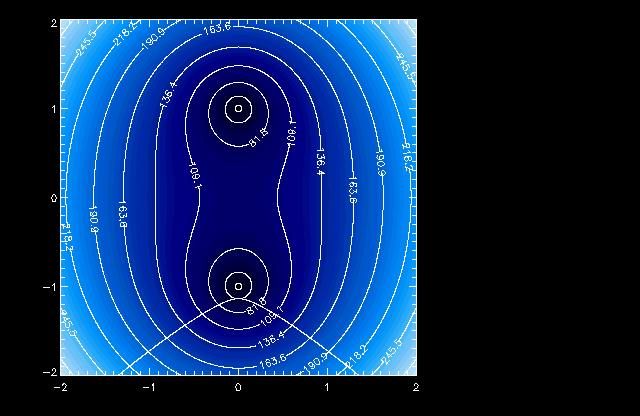
The magnetic field strentgh of the space can also be determined using
Bungey and Priest (1995) if a scaling factor is given. The base of
the flare loop is given a magnetic field strength of 100 G in order
to provide a proper scaling factor. A contour map of the magnetic
field strength mapped below. The characteristic field line that we
will use to describe our loop superimposed.

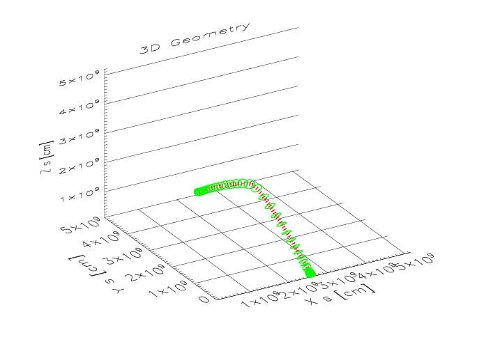
The method described above defines a geometry in 2.5D, with the dimension
coming into and out of the page being redundant. information This is
used to construct a 3D representation of a post flare loop by defining
a circular area at the loop base (or apex) and determing the area
everywhere else by using the constant flux condition.
A rendering of the 3D model is shown below.

Nonthermal Particle
Beams
The beams of nonthermal particles are generated according the
experiment to be carried out. The model beams are comprised of at
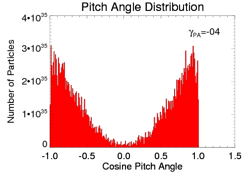
least 2x10^4 test particles. The test particle's initial pitch-angle (the angle made by
the loop's axis and the particle's velocity vector) is drawn randomly
from a probability distribution. For this experiment the distribution
is characterized by a single parameter, gamma_PA. The results from each test particle
are multiplied by a scaling factor in order to represent a true beam
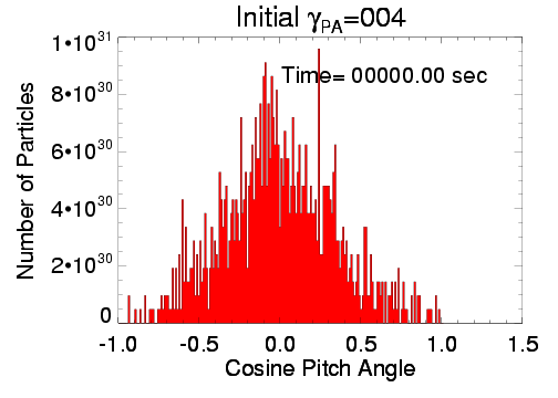
on the Sun. The initial pitch-angle distribution of the nonthermal electrons injected into the
loop apex for a gamma_PA=4 is shown below.

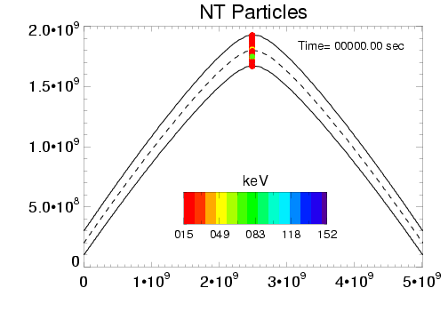
The electron beams are then injected into the 3D flare loop and
allowed to interact with the thermal plasma contained within. The
movie below tracks the position and energies of the particles within
the loop. The particles disappear as they become part of the thermal
distribution.

As the nonthermal particles collide with the thermal plasma they
undergo pitch-angle scattering. The movie below shows the evolution
of the pitch-angle profile.

Thermal Plasma Response
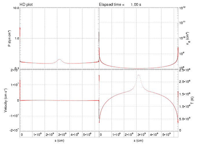
The thermal plasma is defined by three state variables: velocity,
electron number density, and energy density. The benefit of numerical
models is that we can track these variables, and functions of them, as
a function of position and time. The movie below tracks the pressure,
electron density, velocity and temperature.

Simulation Tests
Any numerical model requires an analysis of the simulation's error.
There are many sources of error in numerical modeling. There are
errors related to the precision of the computer and variable types
being used (eg. roundoff errors). There are errors do to limitations of the
numerical techniques used to solve equations (eg. truncation
error). Often, physical quantities that are an integral part of the
model's equations are not well known, or approxiamted by
theoretical constraints, which makes for a source of error that is
nearly impossible to quatify.
Grid Test
Limitations in the number of spatial and temporal grids is also a
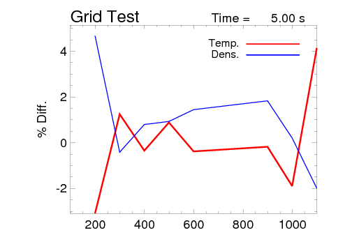
source of error. In order to quantify the "grid error", a simulation
was conducted on a variety of grids. Each simulation used an
identical initial nonthermal particle beam. However, the equations
governing the evolution of the particle beam have stochastic elements,
which will still make for differences in solutions that are not grid
dependent. A series of plots were made, one at each output time step,
that illustrate the effect of spatial grid space size. A
temperature and electron density measurement is made at the apex of
each loop. A percent difference between the measurement made at a
given grid size and its predecessor is plotted and shown below.

The upturn in the percent difference at 1100 grids was unexpected.
Conventional wisdom would have the percent difference decrease as the
number of grids increases. However, the percent difference remains
below 8% for all time yielding an upper bound on the error in the
simulation due to a finite number of grid spaces. Due to time and
computer constraints, a grid size of 700 was used to conduct the
current series of experiments.
Run Tests
Since the nonthermal particles are drawn from random distributions and
the equations governing their behaviour contains stochastic terms,
each run of a simulation will be different. The measurement of these
differences can provide an upper bound for the error incurred by using
a finite number of test particles to represent the entire beam, and a
lower bound for the overall error.
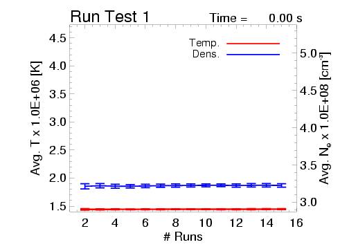
A series of N runs were made, each regenerating a beam from the random
distributions in order to better sample the parameter space. As
before temperature and electron number density are measured at the
loop apex. For the each run from 2 to N a running average value is
made and plotted. Overplotted is the standard deviation of the
average. Additional runs are added until the error is considered
acceptable for the experiment to be carried out.

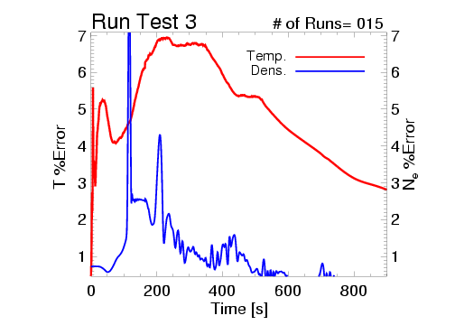
Another useful way to determine how many runs are needed is to plot
the percent error as a function of time for a given number of runs.
No additional runs are necessary when the percent error goes below a
predetermined threshold or when the addition of more runs no longer
reduces the percent error. Below is a plot showing the percent error
of a simulation as a fucntion of time.

Emission Signatures
After a simulation run we have information on temperature and density
for each grid cell as a function of time. The simulation also records
the energy and momentum loss of nonthermal test particles as they
travel through each grid cell. Using this information the emission of
photons from thermal and nonthermal bremsstrahlung can be calculated.
The movie below shows the total emission in the 3-6 keV band in black,
the nonthermal component in green, and the thermal component in red.
The lower plot shows the emission of the viewing area as a function of
time. The imager simulated has a pixel size of 7'' and a Gaussian PSF
with FHWM of 3 pixels.

