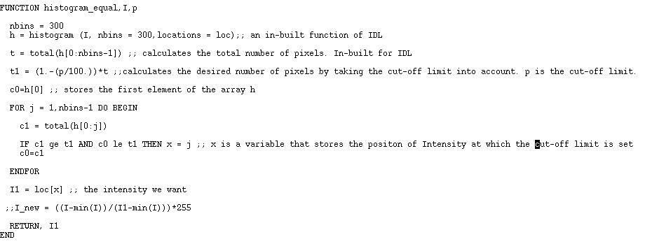
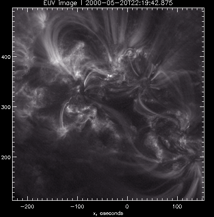
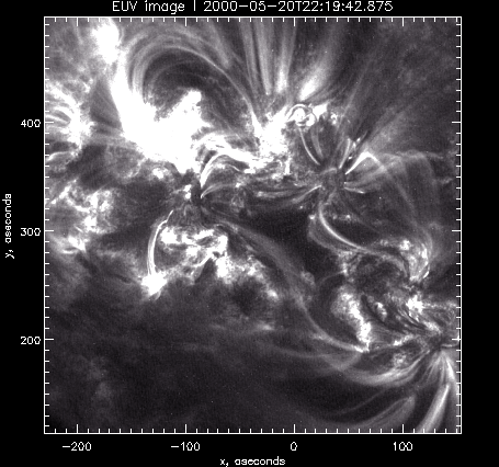
The function is pretty much self-explanatory. As input, the function takes an array containing information about each pixel in the CCD image and a certain percentage of the number of bright pixels that should be discarded from the resulting image. First, it calculates the total number of pixels, t, in the CCD image and then calculates the expected total number of pixels, t1, that should be present in the final image. As output, the function gives back the intensity of the pixel with the maximum value as determined by the cut-off value, p. If the function is implemented, the following result can be seen:
 |
 |
|
Image with normal exposure |
Image with a cut-off value of 5% |
The same day I was also enlightened about the feasibility of using linear force-free model for modelling complex magnetic fields. From the paper "Photospheric and Coronal Currents in Solar Active Regions" by Richard Canfield and Andrew Burnette, I was convinced that the overall twist of the magnetic fields in the active regions of corona and photosphere is essentially the same. They talked about computing α values of the photosphere using three different methods and concluding that they are statistically consistent with the α value of the corona.
June 4th, 2009
The day commenced with the fourth and final IDL tutorial. The topics included reading and displaying images on IDL, adding keywords to programs as user options and so forth. That day I also worked quite a bit on my web journal, and afterwards went through the program my mentor created for me. As I have mentioned before, in a two dimensional image, we can only see loops and is quite hard to predict how the three dimensional magnetic field lines would look like. So the first step would be to trace the loops on the image and later analyze the loops with a computer program that would create a three dimensional magnetic field line judging by the loop we traced on the image. However, my first task was to get familiar with the program that traces the loop on the image. So a short meeting with my mentor later that evening ended the day as I learnt how to use the tracing program.
June 5th, 2009
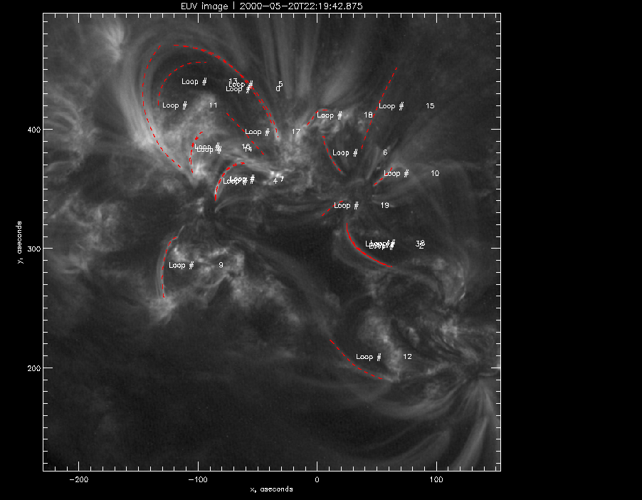
A short presentation on our IDL projects was due that day. After that, I basically played with the loop tracing program the rest of the day. I succeeded to draw around 19 loops and the result is shown below:
|
The execution of the loop
tracing program |
The next step was to execute the program that draws the three dimensional magnetic field lines based on the loops I have traced and that was left for the upcoming week.
Week Two
June 8th, 2009
The next step was to implement the program that would draw the magnetic field lines based on the loops I have traced. However, in order to do so I had to understand the nitty gritty technicalities of the program I was about to use. My mentor had a session with me explaining some useful mathematical tools in Physics such as the Green's function and the delta function. Although I knew about the basics of the delta function, Green's function was a totally new concept for me and later found it as a useful tool to solve differential equations. I learnt that Green's function represents a point response to a phenomenon. If the Green's function is known then the solution to any differential equation can be evaluated using the following formula:
y=∫G(x,x' )f(x' )dx' , where G(x,x' ) represents the Green's function
Using this technique, any magnetic field, B, can be found from the partial differential equation ∇XB = αB, representing a force free magnetic field with constant α. From the magnetic field, the magnetic field lines can be plotted. Whenever α = 0, the Green's function is simple and and the magnetic field can be computed easily. However, the situation gets more interesting if α is something other than zero. Then the Green's function is a function of α and z and plotting the field lines would require more work. In this case, the algorithm has to go through different values of α and z and finding the best values of α and z that would give the minimum value d(α,z) between the traced line and the plotted 3D magnetic field line. Here, d(α,h) is the distance function and the main goal is to minimize it so that we can get as close a representation of a magnetic field line as possible, based on our traced loop. More about the technacalities of the program is discussed in the section Anna's code.
June 9th, 2009
The first of the solar physics lectures was conducted by Dr. Dana Longcope, one of my mentors. The introductory lecture consisted of facts of being sun as a main sequence star in our solar system, how it generates energy and why it is so hot. In exploring energy generation inside the core of the sun, Dr. Dana Longcope pulled topics such as Coulomb's Law and Quantum Mechanical Tunneling from basic physics. The main point of the lecture was that the core was hot because the sun is massive.
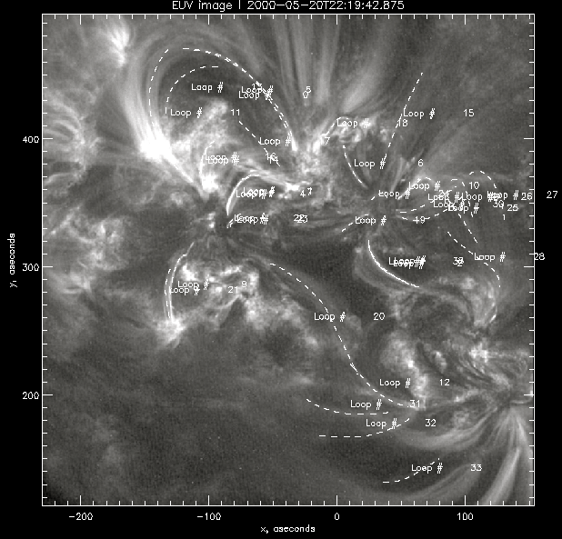
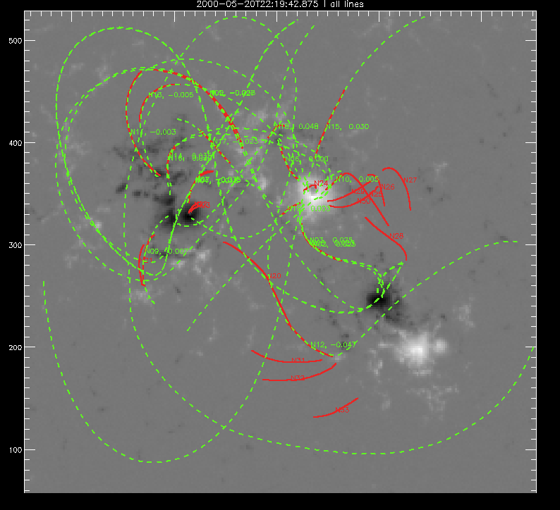
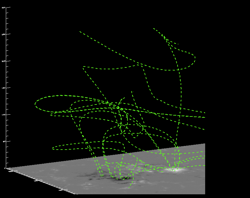
After that, I proceeded to draw more loops on the UV image dated 2000-05-20T22:19:42:875. After drawing the loops, I ran my mentor's magnetic field plotting program. The results are shown below:
 |
 |
 |
Hand-drawn traces |
Magnetic field lines being plotted from the traced loops |
A 3D view |
This was sort of a learning exercise for me as I would have to do it so many times for countless UV images in the upcoming weeks. The loops numbered from 0 to 33 were saved in this file. My mentor also had a reading assignment for me about the way her program works in order for me to adjust to the conceptual complexities associated with the algorithm.
June 10th, 2009
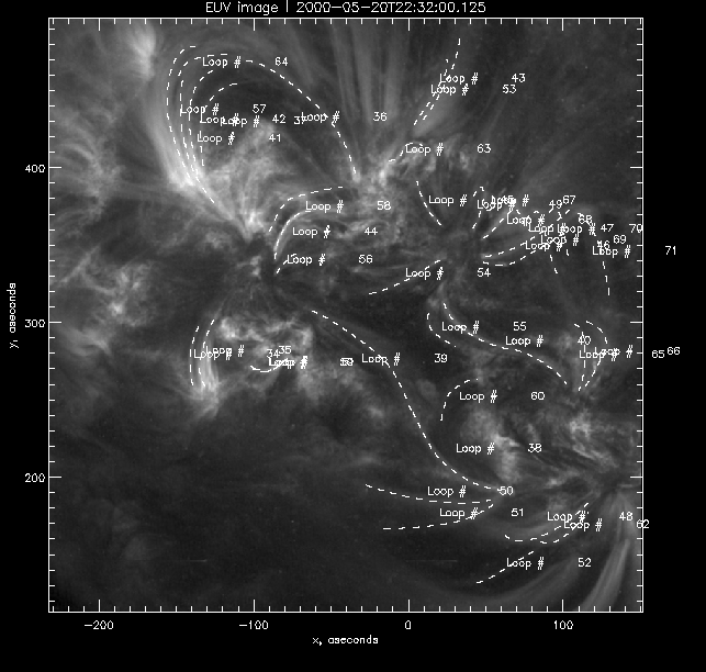
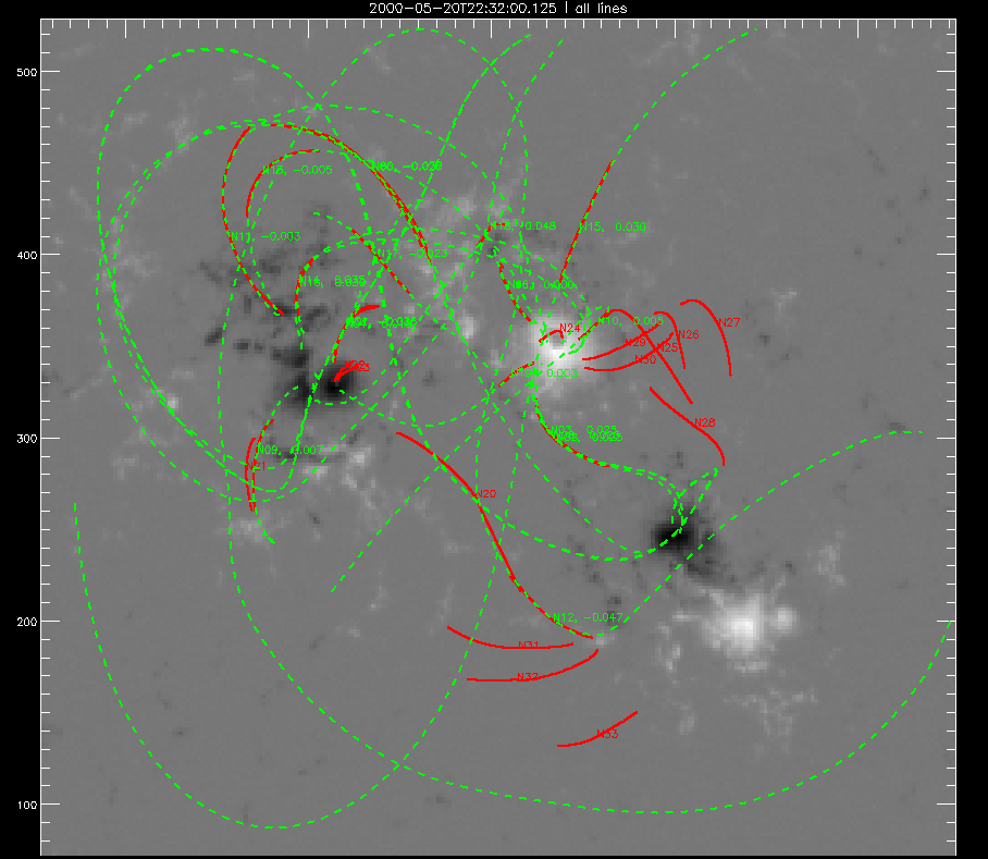
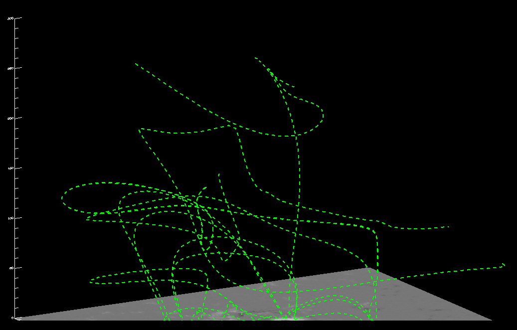
This day I carried on the same routine of tracing and plotting on a different UV image dated 2000-05-20T22:32:0.125. The loops numbered 34 to 71 were saved in this file. This image is taken only 14 minutes after the previous one. The main aim of this exercise was to find out whether the magnetic field changed significantly over short periods of time. As we found out it was not the case and from this we can further conclude that α remains constant over short periods of time. The results are shown below:
 |
 |
 |
Hand-drawn traces |
Magnetic field lines being plotted from the traced loops |
A 3D view |
The previous two plots came out to be almost identical. The exercises of the last two days further goes on to show that, over short periods of time, we can consider the force-free magnetic field model to be consistent with reality. We can hardly see any significant topological changes in the magnetic field of the concerned region.
June 11th, 2009
The second day of the solar physics lectures was conducted by Dr. Kankelborg and dealt with instrumentation in solar physics. He went through topics such as the optical system of solar telescopes, what makes it different from normal telescopes and the special precautions needed to be taken in order to transport it to space.
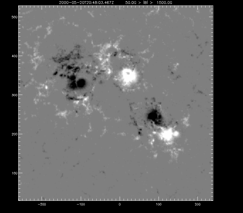
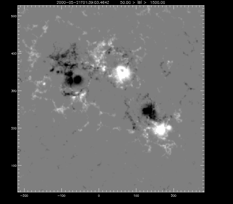
Now that I have explored the topology of magnetic field lines between two closely spaced UV images, I wanted to find out what happens in significantly longer time periods. In order for my better understanding, Anna gave me a file to study - the file consisted of a range of images of the region we were studying. It was particularly interesting to see a sub-region evolving with time and that was our region of interest. My next task was to study that region over some time intervals that were moderately spaced. So these are the four images I was about to study over the upcoming week:
 |
 |
|
2000-05-20T19:12:03.468Z |
2000-05-20T20:48:03467Z |
 |
 |
2000-05-21T00:00:03.465Z |
2000-05-21T01:39:03.464Z |
I am not sure whether it is apparent or not but our region of interest lies in the lower right quadrant of each of these images. Our time frames are quite small, so time evolution of that region is not easily perceivable. However, it becomes obvious over a range of images separated by longer time intervals. The task is to stdudy as many images as possible and see how the α varies in that region of interest.
June 12th, 2009
I proceeded to trace loops on gen 43 dated 2000-05-21T00:00:03.465z . In order to do so I chose two frames of UV images, which were taken plus or minus 20 minutes from the dated time. The selection of the UV images were based on how many visible loops could be seen in a given frame at the given time interval. I found frames 1444.jpg and 1437.jpg to be the ones with the most discernible loops. The .fits file for frame 1437.jpg was 2451685.49325142.fits and loops numbered from 0 to 30 were saved in that folder. Before long, the day was over and the other frame (1444.jpg) was to be traced on Monday of the upcoming week.
Week Three
June 15th, 2009
The day commenced with the third lecture of the solar physics lecture series conducted by Dr. Richard Canfield. The lecture was about solar atmosphere, emission and absorption spectra, the erratic temperature of the solar atmosphere, the different types of solar images and so forth.
After that I continued with my plotting of frame 1444.jpg of gen 43 dated 2000-05-21T00:00:03.465Z . The .fits file for frame 1444.jpg were 2451685.50736310.fits and 2451685.50765593.fits; loops from 31 to 75 were saved in that folder. After that, I executed the magnetic field plotting program on gen 43. There were a total of 75 loops traced for the image gen 43 and so the program was left to run overnight as it would take a lot of computer hours to plot so many fields.
June 16th, 2009
Three other images were left to work with over the week; gen 40, 41 and 44. As I proceeded to work on gen 40, I found no frames for that file on the time interval I wanted. The same thing happened for gen 41. So I started working on gen 44 dated 2000-05-21T01:39:03:464Z. The frames I chose were 1475.jpg and 1477.jpg. The .fits file for 1475.jpg was 2451685.57250602.fits, and loops from 0 t0 31 were saved in that file. Frame 1477.jpg was left for the next day to work with. In the meantime, the field plotting program for gen 43 was still running, and there were 25 more field lines left to be plotted. So, again, the program was left to run overnight.
June 17th, 2009
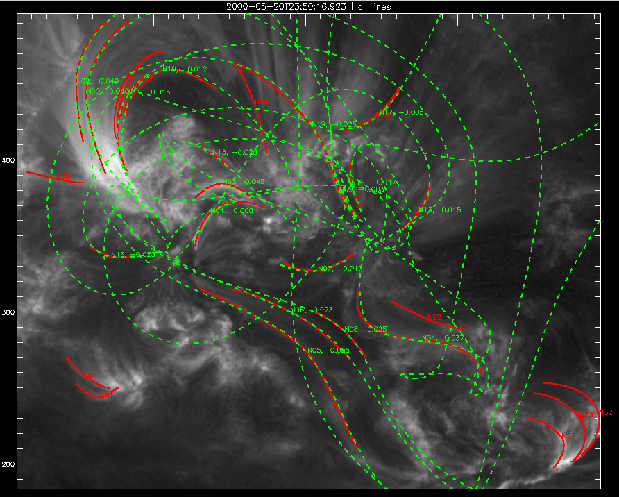
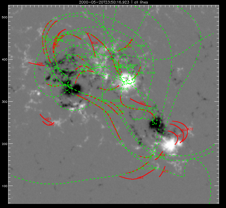
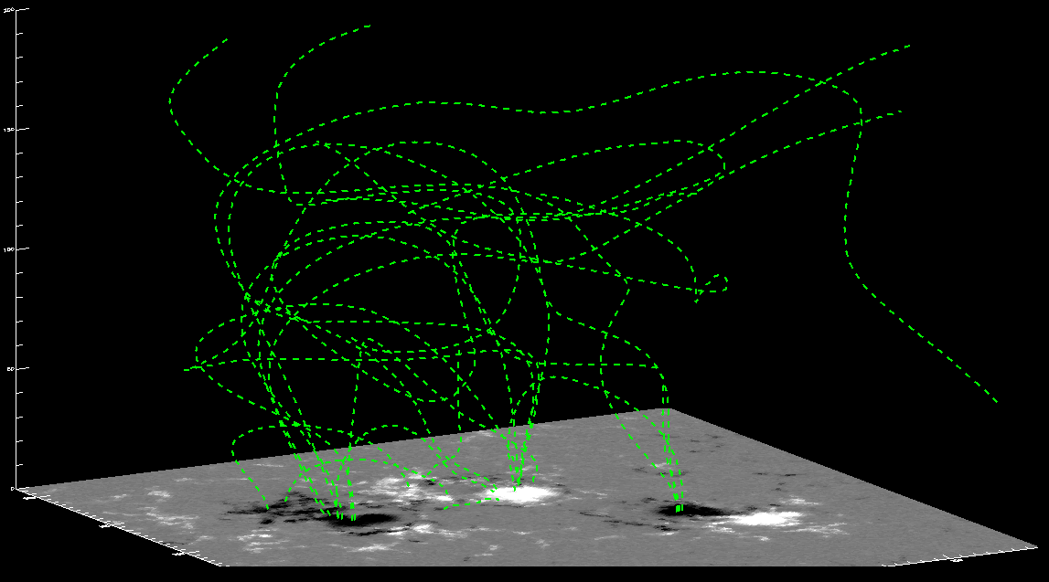
Frame 1477.jpg of gen 44 was tackled that day; the .fits file chosen was 2451865.57707199.fits. Loops from 32 to 58 were saved in that file. In the meantime, the field lines for gen 43 were already plotted. The results for 1437.jpg of gen 43 dated 2000-05-21T00:00:03.465Z are shown below:
 |
 |
 |
UV image with the field lines superimposed on the traced loops |
The same image with the sunspots |
A 3D view |
Showing all the images is redundant and beyond the scope of this page. However, the point I want to make is the region consisting of the two sunspots in the lower right quadrant of the image. Clearly, they have evolved with time as expected as the topological changes in that region is evident.
June 18th, 2009
This day I started working on gen 45 dated 2000-05-21T03:15:03.463Z. The frames chosen were 1511.jpg and 1488.jpg. The .fits file for 1511.jpg was 2451685.64730519.fits; loops from 0 to 30 were saved in that file. The .fits file for 1488.jpg was 2451685.59976701.fits; loops from 31 to 57 were attributed to that folder. So, I drew a total of 57 loops that day.
June 19th, 2009
The fourth solar physics lecture by Dana Longcope was a continuation of his talk about the interior of the sun. He talked about the convective zone, the radiative zone and the mechanism by which magnetism exudes from the active regions.
After that I ran the field plotting program for gen 44 and worked on my webpage a bit before it was time to go to the Yellowstone star-gazing trip.
Week Four
June 22nd, 2009
I ran the field plotting program for gen 45 and proceeded to read a paper written by my mentor giving a detailed analysis on the way her algorithm works. More about this is discussed in the section Anna's code. Through this reading, I had a better understanding of what the field plotting program was actually executing on my screen. I also learnt about the feasibility of using constant α field model for approximating fields where the α is not constant. I found that, within statistical limits, it is not a bad approximation at all.
After that, my mentor gave me an exercise to deal with situations when the line of sight is not straight forward. If the line of sight is different other than directly in front of the observer, then we have to express the new line of sight in a different coordinate system. This we can do by using the various transformation matrices we learn in linear algebra.
The field lines as plotted by the program, although does a reasonable job, is not totally accurate. In order to get a better representation of the magnetic field lines, it is necessary that the bad lines are discarded. For that, we have to manually fit the lines that would give a better fit than the computer plotted lines. This is what I am about to do next, and I start with gen 43 dated 2000-05-21T00:00:03.465z.
June 23rd, 2009
The fifth solar physics lecture, by Sylvia Guidoni, was very informative for me as she talked about the nature and origin of the sun's magnetic field. She stressed on the Zeeman effect, which was the key to understanding the origin of the magnetic field emanating from the sunspots. In an attempt to elucidate the concept of Zeeman effect, Sylvia brought forth the quantum mechanical model of the hydrogen atom and the different properties associated with it. Zeeman effect is only possible in the presence of an external magnetic field, hence the Zeeman splitting of the absorption lines from the sunspots gives credence to the inherent magnetism evident in the sunspots. Why are we so much concerned about the Sun's magnetic field? The answer lies in accurate space weather predictions, which is the key to understanding GPS and other telecommunications failures.
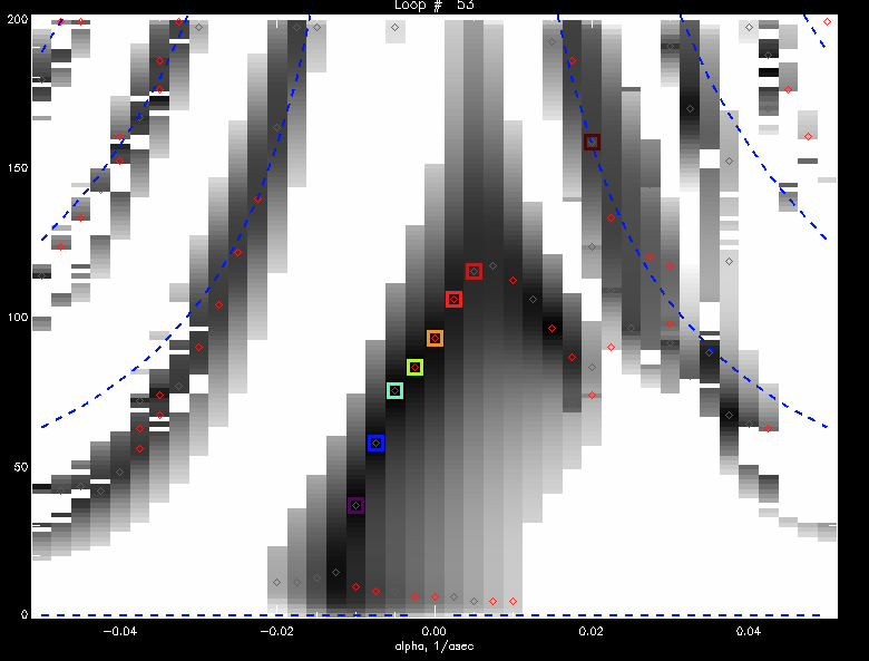
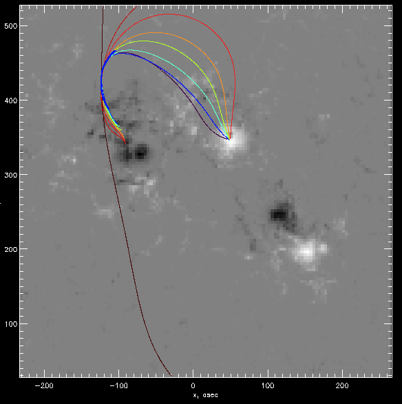
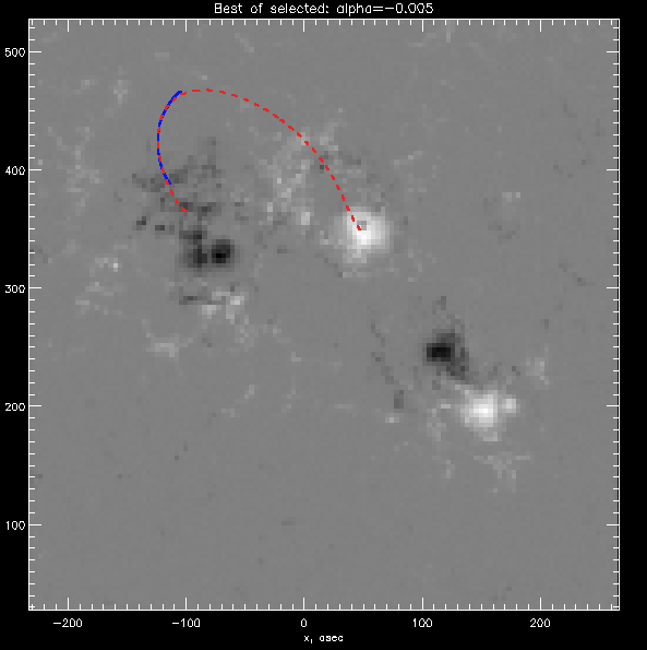
As promised, I started working on manually fitting the magnetic field lines of gen 43. The following diagrams may be helpful in illustrating what I did:
 |
 |
 |
|
The parameter space |
The best possible loops |
The best loop |
The picture on the left is the parameter space. The x-axis represents the α values, y-axis represents the h values; h is the point in space where we extrapolated the traced loops to make a 3D magnetic field line. The distance function d(h,α) represents the distance between the traced loops and the auto-fitted field lines, which we got by running the field-plotting program. Our aim is to get the minimum d(h,α) between each traced loop and the corresponding field line. The dark and bright pixels represent minimum and maximum d(h,α) respectively. However, from the parameter space, we can see that there are many possible field lines that can be plotted for any given traced loop. There are many dark pixels indicating that there can be more than one field line that can be plotted for any given traced loop. The auto field plotting program choses a minimum point (minimum d(h,α)) indiscriminantly, usually based on the darkest pixel. However, this tactic does not always give the best fit based on the trajectory of a loop. All the darker pixels are marked with red squares; manually selecting them would give us a range of values of d(h,α). Then, we have to select the minimum value of d(h,α), which has the lowext h value. The middle picture shows all the possible field lines for our chosen points and the right picture shows the field line that we finally selected manually. Selecting the points from the parameter space is still a subject of investigation. Usually, the structure with the two arms meeting (as shown on the left picture) is the most interesting region for choosing the points. The structures which look like hyperbolas are definitely not good options for selecting the points. We do not know the explanation yet, but that's what works for now.
I finished manually fitting gen 43 and my mentor pointed out the discrepancies between my and her results. I noted them down and left them for the next day to work on along with the manual fitting of gen 44 dated 2000-05-21T01:39:03:464Z.
June 24th, 2009
The discrepancies between mine and Anna's manual fittings were based on comparing the α values for each field line. For gen 43, we found 20 out of 57 field lines with discrepancies and it was a learning exercise for me to choose the apt minima from the parameter space that would give a proper representation of the field lines. The selection of minima from the parameter space was kind of arbitrary and depended a lot on the selector's judgement. Since it was Anna's algorithm, she had a better insight of what needed to be done and I just followed along with her algorithm. After gen 43, I dealt a bit with gen 44 before quitting the day.
June 25th, 2009
The sixth solar physics lecture by professor Jiong Qui dealt with solar magnetism from a more mathematical perspective. She mentioned about the twist in magnetic field, magnetic reconnection and coronal heating. She used the Ampere's Law in good effect in making us understand the mathematics behind magnetic reconnection, joule heating of solar corona and so forth. All in all it was a good and enlightening lecture.
I finished manually fitting gen 44 and this time the results looked encouraging; I had far fewer discrepancies with Anna's manual fittings. After that, I had a session with Anna discussing our future course of action. She instructed me of postponing manually fitting the field lines for gen 45 and showed me two loops I traced from two different frames of gen 45. She believed that those two loops were from the same source but were separated in time. We found out how far in time the xrt images were from the actual magnetogram and how far the xrt images (2451685.64730519.fits & 2451685.59976701.fits) shifted, in arcseconds, with respect to each other. We found the shift to be approximately 7 arcseconds in the x direction. After that we shifted loop # 32, of 2451685.59976701.fits, seven arcseconds and found out that the shifted loop had approximately the same α value for the manually fitted field line, but a different h. After that, I shifted loops numbered 31 to 57 of gen 45 and assigned the the numbers 61 to 86 for the shifted ones. Then I started the auto field plotting program for the shifted loops.
June 26th, 2009
My mentor needed more data for xrt images that were closer to the disk center and advised me to trace loops for gen 38, 39 and some more frames for gen 45. For gen 39, frames 1311.jpg and 1318.jpg were selected. For frame 1311. jpg, the TRACE image was 2451685.23085740.fits and loops from 0 to 43 were traced on that image.
On the weekend that followed more loops were traced for gen 39. For frame 1318. jpg, the TRACE image was 2451685.24513865.fits and loops from 44 to 82 were traced on that image.
Week Five
June 29th to July 2nd, 2009
Week five was basically tracing lots and lots of loops and also manually fitting the field lines. For gen 38, frames 1275.jpg and 1280.jpg were selected. For frame 1275. jpg, the TRACE image was 2451685.15528865.fits and loops from 0 to 33 were traced on that image. For frame 1280. jpg, the TRACE image was 2451685.16572441.fits and loops from 34 to 62 were traced on that image. Another frame that was chosen for gen 45 was 1509.jpg; the TRACE image was 2451685.64273343.fits and loops from 129 to 165 were traced on that image.
The first of the lectures of Professor Eric Priest was delivered that week. It was basically a revision of what was already stated by the other lecturers so far. He talked about the solar atmosphere and the basic structure of the sun.
Week Six
July 6th ,7th, 8th, 2009
The second lecture of professor Eric Priest dealt with the derivation and application of MHD equations. It was a concise and rough overview of what MHD was all about.
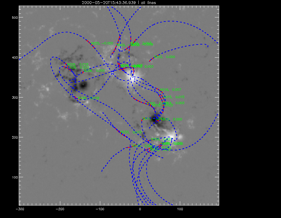
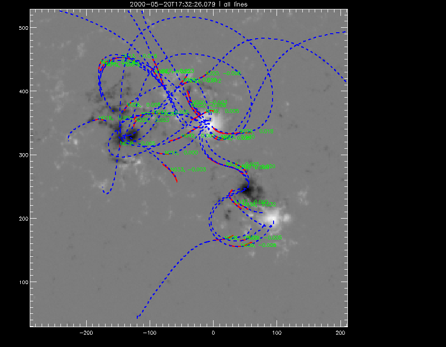
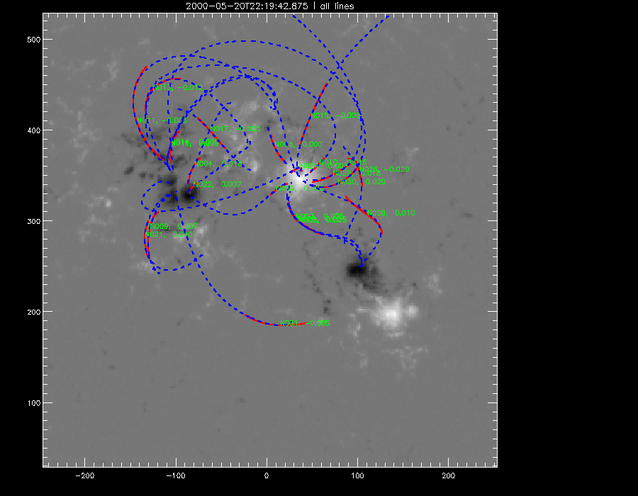
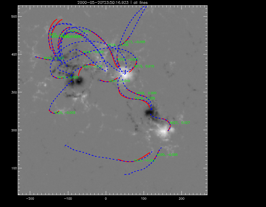
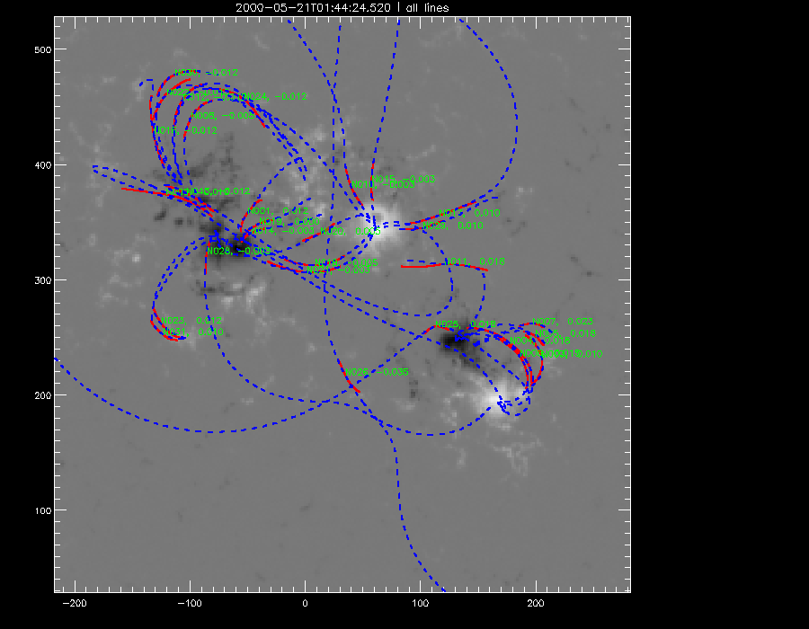
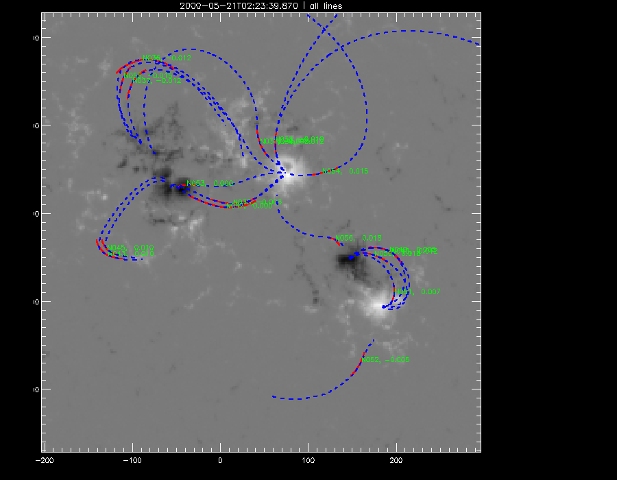
The last of the manual fittings were done. Here is my data as of yet containing information of all the TRACE images done so far. All the manual fittings with a quality less than or equal to 0.5 were discarded. Shown below are some of the magnetograms with the 'good' fittings of the various mdi s attempted so far.
 |
 |
|
gen 38 (2451685.15528865.fits) |
gen 39 (2451685.23085740.fits) |
 |
 |
|
gen 42 (2451685.43035735.fits) |
gen 43 (2451685.49325142.fits) |
 |
 |
|
gen 44 (2451685.57250602.fits) |
gen 45 (2451685.64730519.fits) |
So now we have data spanning over a few hours starting from 2000-05-20T 16:00:03.470z of the magnetogam gen 38. Between gen 38 and gen 45 there are 11.25 hours. The next step is to analyze the data, especially of the two dynamic poles in the lower right quadrant of the images. One way to do so is to assume that those two poles constitute a bent force-free cylinder, with the magnetic field lines on the surface of the cylinder. As the two poles rotate around each other and also about their axes, they create twists in the magnetic field lines as quantified by the alpha values over time. From theory, it can be derived that the relationship between angle and the overall twist is Δθ=0.5αL, where L is the length of the field lines in arc seconds. Empirically Δθ = Δθ(positive pole) + Δθ(negative pole) + Δθ(rotation), where Δθ(positive pole) is the rotation of the positive pole about its axis, Δθ(negative pole) is the rotation of the negative pole about its axis and Δθ(rotation) is the rotation of the poles with respect to each other. When I calculated the angle for gen 39, for instance, the theoretical and empirical values turned out to be 0.29 radians and -0.834 radians respectively. Clearly, they are not the same as expected and makes us wonder whether our force-free model is compatible under dynamic circumstances.
July 9th, 10th, 2009
For a better illustration and convenience of addressing let's number the loops we have in the trace image. Here's what we have:
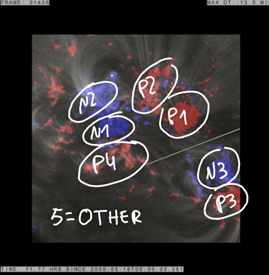 |
The trace image shows the various positive and negative poles in our region of interest. P stands for positive and N stands for negative. P1, P2, P4, N1 and N2 remain relatively static compared to N3 and P3, which is our main region of study. |
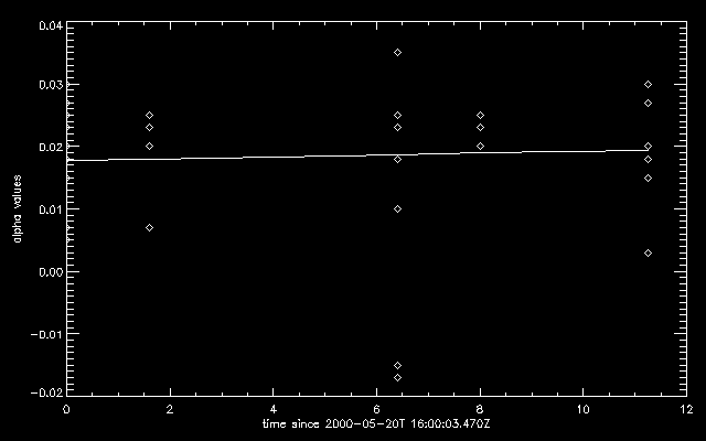
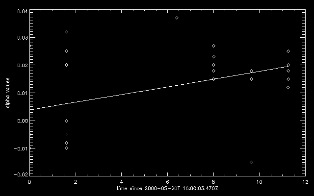
A plot of α values with respect to time gives us more insight about the limitations of our algorithm. Given below are the two plots of α values against time for the field lines going from P3 to N3 and P1 to N3. The time of reference was taken to be that of gen 38 dated 2000-05-20T 16:00:03.470Z. P1 and N3 remain reasonably stationary relative to each other compared to N3 and P3, which are seen to evolve with time.
 |
 |
|
P1 to N3 |
P3 to N3 |
For P1 to N3, we can see a consistency in the α values with time; not so much for P3 to N3. Least squares fit was applied to each of the plots, and we can clearly see that our algorithm agrees with what was expected i.e. α remains almost constant for the 11.25-hour period for the region (P1 to N3) which is not that as much dynamic as the one which is dynamic (P3 to N3).
Week Seven
June 11th to 17th, 2009
Lots of loops were traced this week as we needed more data for times approximately 30 hours earlier than gen 38. Here is a table of what I did:
| mdi |
frame |
TRACE image |
Number of loops |
| gen 20 (also manually fitted) |
634 639 |
2451683.82063005.fits 2451683.83105250.fits |
0 - 41 42 - 74 |
| gen 29 |
956 965 |
2451684.49133630.fits 2451684.50966210.fits |
0 - 46 48 - 96 |
| gen 22 |
703 709 |
2451683.96483718.fits 2451683.97722663.fits |
0 - 35 36 - 77 |
| gen 25 |
827 833 |
2451684.22255976.fits 2451684.23474436.fits |
0 - 29 30 - 68 |