Home
Resume
Daily Journal
Anna Malanushenko's algorithm
Final Presentation


Anna's Algorithm

My mentor Anna has developed a unique algorithm to model magnetic field lines, based on the primary assumption that the field is force free. Whenever we look at a TRACE image in extreme UV, we can discern loops that are apparently magnetic in nature. However, the loops give us very little insight about the topology and characteristics of the actual magnetic field lines. So plotting the magnetic field lines become necessary in order to get a better understanding of the magnetism in the active regions.


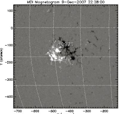
          Active region with the sunspots as seen in a magnetogram
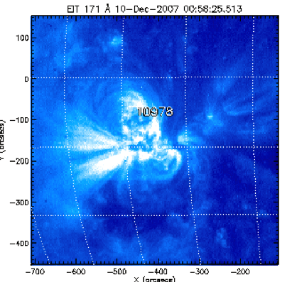
                The same active region in extreme UV

As we can see above, the magnetogram shows the sunspots with their respective polarities and the extreme UV image shows the magnetic loops. So, given the loops, we can trace them on the TRACE satellite images in order to give them a more visible and distinguishable outline. From the traced loops we know the x and y coordinates, and depending on whether or not we know the magnetic field for that loop, we have to adopt different techniques in order to plot the magnetic field line for that particular loop.


First case - suppose the magnetic field is known

Just a review of the force free magnetic field equation, which can be written as
∇XB = α B
. By known magnetic field, we mean that it is easily calculable and is only possible if α = 0. The procedure can be explained as follows:


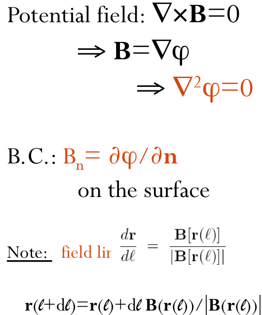
                        The underlying math
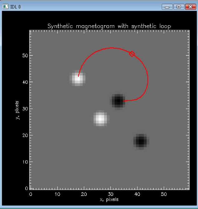
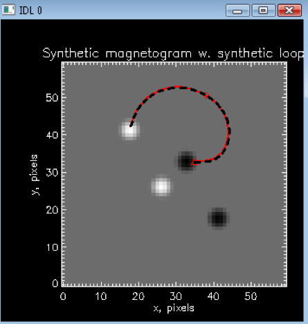
                                        The loop
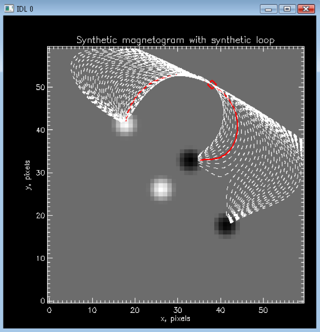
                      Many possible magnetic field lines


The magnetic field can then be expressed as just the gradient of a potential, which can be further expressed as Laplace's equation. The partial differential  equation that results from all this can be solved analytically if the boundary conditions are known. After the magnetic field is known, plotting the field lines would be trivial.

As we can see, the solitary loop is just a possible field line in the x-y plane. If we pick a point on the loop, we know (x,y) but not z. So if we try different values of z for the same (x,y), there will be an array of possible field lines. Ok, now that we have so many possible field lines, what to do with all of them?

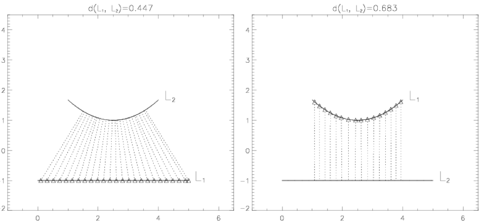
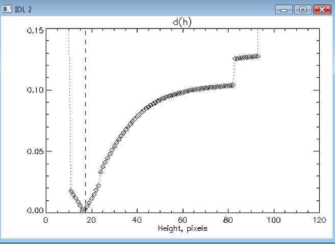
The idea is to find the distance between each field line, L2, and the traced loop, L1, and pin-point the field line that gives the minimum distance, d(L1,L2). The resulting field line that would be obtained would be the one with the best h-fit or z-fit, whatever one calls it. The distance function d(L1,L2) has to be assigned; it basically represents the mean length between points of one curve, L1, and the whole of second curve L2. One thing that has to be kept in mind is that d(L1,L2) and d(L2,L1) are non-commutative. The illustrations are shown below:


             Non-commutative property of d(L1,L2) and d(L2,L1)
                 Best h-fit occurs at minimum d(h)
                           The best fit


Second case - suppose the magnetic field is unknown with constant α

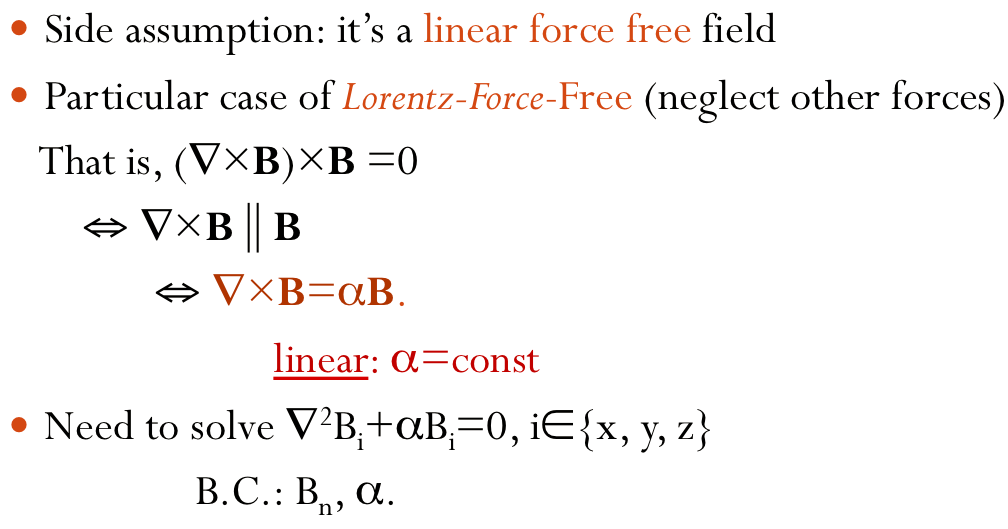
If the magnetic field is unknown, it means that we don't know about α. The primary assumption would be that the field is linear and Lorentz force-free. If that's the case, then the following is true:

As we can see, there are two unknowns in this case, B and α. So this results in a partial differential equation that is linear and easily solvable for B , if α and the boundary conditions are known. The fact that the field is force-free makes it useful in modelling magnetic equilibrium, and also the linearity makes it easy to compute. 

Since both α and h (or z) are unknown, distance between the traced loop and the corresponding field lines would be a function of both α and h. So the minimization d=d(α,h) has to be done in (α,h) space.

The following steps are needed to be executed:
  • Different α s are tried as α is unknown.
  • For each α, the best-fit h is selected.
  • The "best-fits" for different α s are compared and the best is taken.
  • Best is the one with the minimum d(α,h).
This method works exceptionally well for constant α fields and is an efficient means of finding α for a given magnetic field line.


Some of the illustrations of the algorithm are shown below:
                                         The underlying math


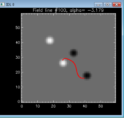
                                     One loop
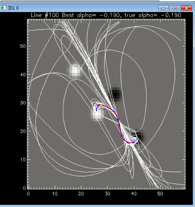
        Many possible magnetic field lines


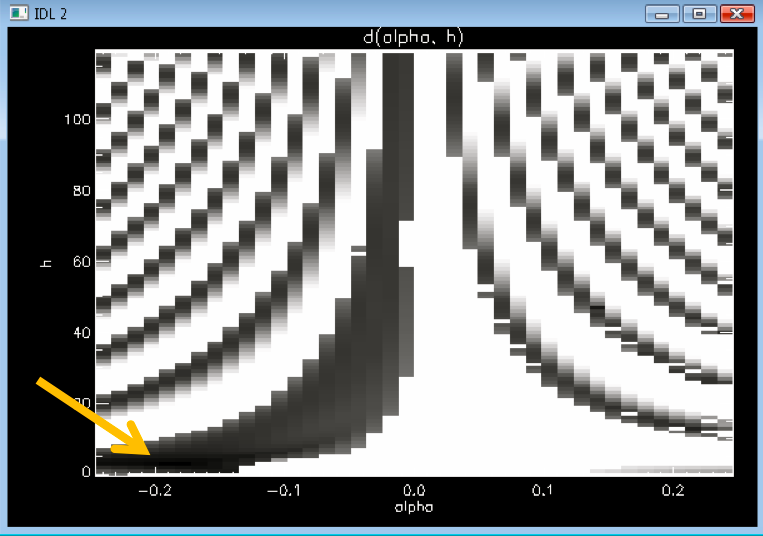
  Parameter space - dark pixels indicate minimum d(α,h)
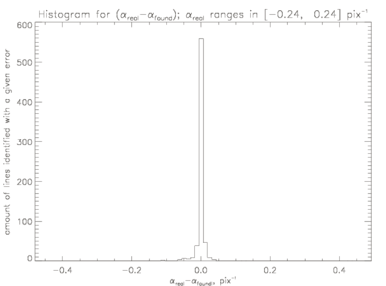
                        Accuracy of the algorithm


The algorithm can also give us a very good approximation about non-constant α fields. In that case, the magnetic field would be hard to compute as the resulting partial differential equation would be non-linear.


                                                                                                                                   Previous