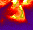
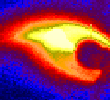
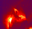
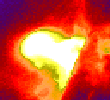
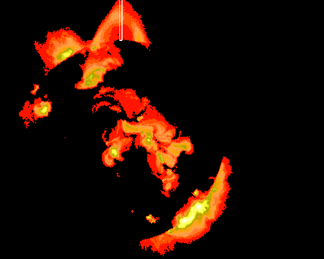
First, images were created from the four main flares. These flares are dated with time spans: January 24, 1992 (09:11-22:43); February 21, 1992 (03:10-14:50); April 22, 1993 (17:19-04:00); and March 22, 2001 (17:20-17:30). (See flare images below respectively.) The January 24 and April 22 flares were observed only in full-sun images. The February 21 and March 22 flares were observed in partial-sun images. The raw data for these flares was obtained using the week directories in the Yohkoh data archives. The program .run yodat was used to obtain this data in the relevant week directory number. For each flare, two images were made from an arbitrary frame number which has a specific time. Color tables were chosen for the images, e.g. std gamma-II and red temperature, and the gamma correction was lowered in order to show more detail and clarity in the flare. These images were created as .gif files from the command 'write_gif'.


Next, movies
were created for each flare. The program image2movie was used to create
.gif and/or .mpg movie files. Each movie was made from a select number
of sequential frames. The number of frames could have been selected manually
by assigning a variable to a string of listed numbers, or as a data set
within a certain range. As with the images, an appropriate color table
was matched with each flare due to clarity and visible detail.
The programs
rebin and congrid were used to change the size of the array in flare images.
This was used to make the image appear at a larger scale, so as to view
better.
Then, raw
flare images were prepped. The prepping procedure could be carried out
manually or through the program sxt_prep. Mainly the prepped data was completed
by sxt_prep. This program was used for the two partial flares of Feb.21,1992
and Mar.22,2001. Just before running sxt_prep for the two partial sun flares,
the raw data was selected by .run yodat and then sswhere was used to set
the parameters for the raw data that was chosen. In sswhere frame completeness
was 100%, zero saturation of pixels, modes were normal, DP modes were quiet
and flare, full resolution, compressed, A filters open, all B filters,
all DPE values were chosen, and finally the field of view was selected.
The arrays that came from this selection
contained all the images to be prepped for the flare.
In sxt_prep
many corrections are performed. The raw data was decompressed with its
uncertainty. A measure of the dark data was taken and then the dark current
was subtracted from the out data. A measure of stray light/leak data was
taken and subtracted, if needed, from the out data also the exposure duration
was normalized. The images were also aligned. Each of these steps were
completed through the standard program of sxt_prep. In addition, the program
sxt_dn_unc was run after sxt_prep in order to consider the remaining uncertainty
due to photon counting statistics.
Next, "bad"/unwanted
frames were removed from prepped data. The unwanted frames were listed
by number in a variable string. 'Kill-index' was used to get rid of the
"bad" frames and keep the remaining ones.
The two remaining
full sun images of Jan.24,1992 and Apr.22,1993 were prepped using the program
sxt_prep also, but they required an additional correction. The long and
short exposures had to be combined to get rid of saturation in the images.
All of the corrections previously mentioned for the partial flares were
carried out in the same manner for these two flares as well.
After each
flare was prepped with all its data, then another initial preparation was
completed for each allotted filter. This separated the prepped data by
each "B" filter that the flare data was taken in. The prepped data then
was rotated so that the flare of interest was at the top, center of the
image window. The 'rot' command was used in rotating the images. Also,
the uncertainty that was associated with the prepped data was rotated to
the same degree using the same technique. I decided to rotate the images
by a relative integer amount, according to an estimation of how it looked
in the image window. I decided to rotate by these amounts: Jan.24,1992,
225 degrees; Feb.21,1992, 70 degrees; Apr.22,1993, 44 degrees; Mar.22,2001,
65 degrees. I developed a program that could rotate the group of images
instead of doing it manually. It is called mk_regrot.pro.
Next, I took
the differences between the frames. Differencing is a technique used to
accentuate changes in the flare between image frames taken over time.
I used the 'where' command to find the images in the specific "B" filter.
I carried out the subtraction in the array of images that were needed.
The subtraction was completed using 'safe_log10' of the data out because
this seemed to be the best output option for subtraction of frames. Then
the subtracted data for each flare was rotated in each "B" filter, especially
in the filter with the highest amount of frames. The subtracted data was
also rotated to the same degree as the initial prepped data without differencing,
respectively. This was done using the same technique with the 'rot' command
mentioned earlier. In addition, the rotation of the subtracted data was
completed in the "B" filter with the highest amount of frames as well.
Then, using the
rotated data in the "B" filter with the highest number of frames and using
the rotated data of the differences in the same "B" filter, stack plots
were made. The stack plots can be obtained by using a manual method or
the program mk_stack.pro. A slice of single column pixels was taken from
the estimated center of the flare. Then that slice was taken out of the
exact place from every frame in that same array. Then the slices were lined
up next to one another in order to create a stack of slices from each frame.
Also, the stack was saved as a .gif image through 'write_gif' in order
to make it easy to view in xv. A different type of stack could also be
made through a normalized byte scale of the data using a minimum and a
maximum brightness. However, this method was not performed and saved on
all flare files.
Then, the
program sxt_teem was used to create maps of temperatures and emission measures
for all four flares. First, one image was made from two frames that came
from two different filters. Sxt_teem outputs the temperature, emission
measure and the uncertainty for the target area in the image. After sxt_teem
creates the image, then the temperature and the emission measure can be
altered according to clarity and dark/light composition by the minimum
and maximum values. 'Ocontour' can then be used to create a contour map
of the flare in the image. An additional program can be run to create a
color scale that can be placed onto the temperature map.
In order to
obtain two filters from each flare, considering that some have multiple
filters, I used the rotated data files that contained all possible filters.
This supplied an easier route to obtain the data to run sxt_teem. However,
an alternate program had to be created because sxt_teem would not include
several images in two filters, or pull data from the index of only two
numbered filters. The program teem_movie.pro was the solution. The
temperature and emission measure movies created from this program are also
referred to as color movies. With this program the data could be
obtained from a certain filter in a certain range of frame numbers. Also,"bad"
frames that did not match up in time or provided too much of a time gap
could be removed from the index of data. Temporary arrays were made in
order to provide a certain range of data that was comprised of at least
two different filters. 'Kill_index' was run in order to remove any "bad"
frames. Then, teem_movie created a movie of new images that were from two
different filters and paired to match closely in time. The preferred time
span was a few seconds, but larger time spans had to be allotted for certain
flares. The temperature (te) and emission measure (em) were adjusted for
minimum and maximum values and saved as mainly n_temp or n_em.
A different
amount of temperature and emission measure movies made by teem_movie were
completed for each flare. One movie was made for the Jan. 24 flare and
the Apr. 22 flare. Both were created in filters 2 and 3. Several movies
had to be created for the Mar. 22 flare and the Feb. 21 flare because of
the amount of filters in the data and the arrangement of the data gaps.
Filters 3,4, and 5 were in the data for the Mar. 22 flare. Five temperature
movies were created with different combinations of those filters and in
different ranges of data in the index. For the Feb. 21 flare filters 2,3,4,
and 5 were present. Six temperature movies were made to incorporate different
combinations of those filters and in different ranges of data.
From these
temperature movies stack plots could be made for each flare in each pair
of filters. The program mk_stack2.pro was run in order to make a stack
from the number of images in the data set from teem_movie. The initial
stack for each flare was made from each different temperature movie and
contained slices that were one pixel across and a range of y values tall.
The stacks that were made for each flare were saved as a .sav file and
as a .gif file. The first temperature movies and stacks were made in the
black and white color table, and adjusted accordingly. The x and y coordinates
for each stack were documented and used for similar stacks for the same
flare. This on the left is the April 22 flare at the very top of
this image with the line drawn in white of where the stack of one pixel
wide was taken from. On the right is the January 24 flare at the
top with the stack outlined in five pixels wide.

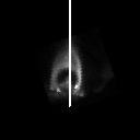
This is the stack plot of the regular data for the April 22 flare in one pixel width.

The next step was to manipulate the mk_stack program to include several pixels across, not just one single pixel wide, so as to view more data and how it changed over time. This was especially useful if the flare became curved over time or if the orientation was different at different times. This program was called mk_stackwidepix2.pro. It uses the same functions as mk_stack2.pro, but it adds 2 pixels to each side of the average pixel on the x-axis. Therefore, there is a total included range of 5 pixels on the x-axis. This program for wide pixels was applied to all the flares and performed on the same data that was used to make the single pixel program. The following image is of the stack plot of five pixels wide for the April 22 flare.

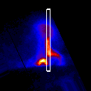
For the single and wide stacks of the flares, images were made that showed a single frame of the appropriate data set and an outline on top of it of where the stack was taken from. A single frame was chosen of a flare and displayed on the screen. Then, a variable was defined within the space of the image and assigned the proper x and y coordinates. When this variable is used with the 'ocontour' command it produced a line or box, according to pixel size, that was brighter than the rest of the image. Then the image with the line or box on it was saved as a gif file after doing a 'tvrd' for the onscreen image. See below images with stacks outlined for Feb. 21 flare in one pixel wide on the left and on the right five pixels wide.
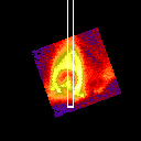
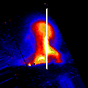
The images below are of the March 22 flare with stacks outlined of one pixel on the left and five pixels on the right.
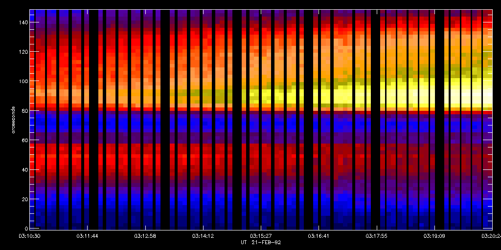
Below is the stack plot with tick marks for the April 22 flare regular data with a pixel width of five.
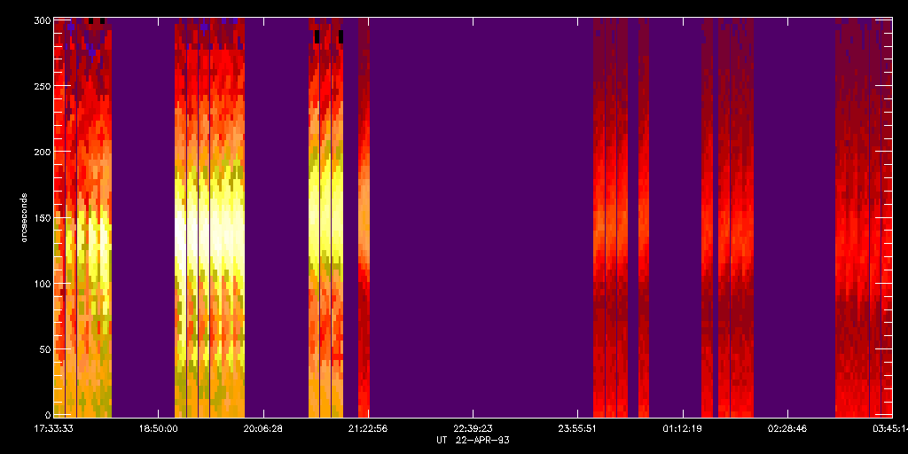
An alteration
needed to be performed on the program mk_stacknew_ticks because the April
22nd flare had data from two different days. This program was called mk_stacknew_tickstimes.pro.
This program had to be created because it would not create the stack or
display the proper times on the second day. Within the program the times
of the second day had to be altered by adding 24 hours (86400 seconds)
to them to allow the times of the whole data set to gradually increase
with the increasing number of frames.
An additional
program was needed to redisplay the stack made with time ticks from mk_stacknew_ticks.pro.
Plot_stackticks.pro was the program name made to read the info from mk_stacknew_ticks
stored in the stack variable and output the stack with time ticks. The
input requires an index, the stack, a /nosq, and a width parameter. This
would be very useful in looking at the stacks with the proper tick marks
of time for the final analysis.
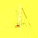
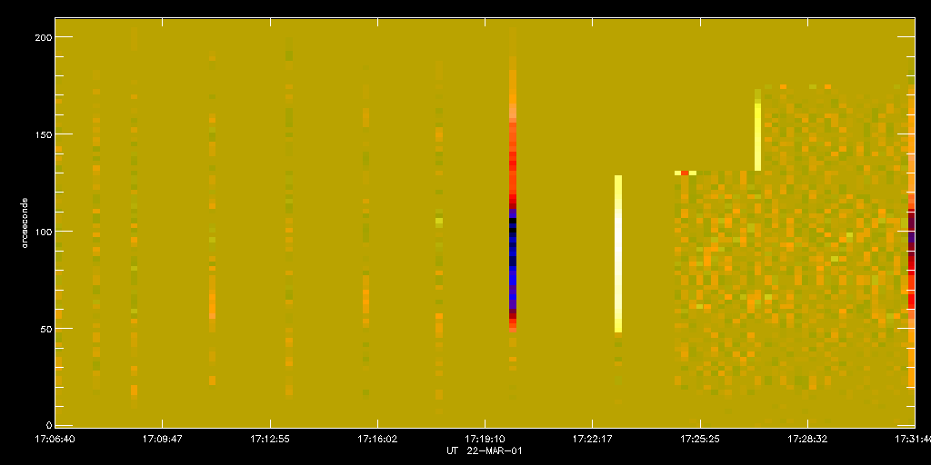
Below is an example of the subtracted data. This is the March 22 flare on the left from the subtracted data. On the right is the graph with the time ticks of the stack plot of the subtracted data in one pixel wide.
Top of Page
Back to Main Page
Background
Previous - Info
*My Project
Next - Programs
Results