---

7th June 2010 Today is the first proper day of research, and so I began the first part of my project, which is to perform some analysis of the magnetic reconnection of the 15th January 2005 Flare, which can then be compared to the Hard X-ray analysis of the same flare, to investigate the two ribbon problem. I will be measuring the spatial evolution of the region by first measuring the reconnection rate as a function of time, and then the physical dimensions of the ribbons evolve. During last week's IDL Assignment I found that the median's of most of the time frames were negative, suggesting that a large proportion of the whole data set had negative values. During the data correction process from satellites such as TRACE (i.e. an instrument with a CCD) a dark current is subtracted, and in this case, it appears as though the dark current was not the correct value. A CCD is a collection of semi-conductor pixels, and when a photon impacts a pixel, it displaces an electron from the surface. These ejected electrons are then measured via a current, and so a dark current is a current present in the pixel when no emitting object is in the FOV (or at least, no significantly bright object). In the case of the TRACE data I am using, this dark current probably changes with exposure time, meaning that a single correction factor is not appropriate and caused the large number of negative values observed. My first task is, therefore, to re-correct the data. Jiong is pretty sure that the dark current is time-independent, so a linear relationship with exposure time (I got a bit confused for a while between the time, and then the exposure time). If this is the case then the solution is pretty simple. If not then I guess we'll cross that bridge when it comes. To test the dark current relationship with exposure time I was given a program which I had to adapt to work with my flare. This was quite useful as it meant I could get used to using IDL without having to write my own program. If linear then the observed median, M', would be related to the initial dark current correction, DCo,  the median value of the ith frames, M(i), and the  ith exposure time, Texp, by : M' = (M(i) - DCo) / Texp(i) Then if the true median value, M, and DC the actual dark current correction to be applied, then M' can be given by: M' =  M - DC/Texp(i) and so M' ~ 1/Texp. The plot below shows a remarkably linear relationship:

Medians Vs 1/Texp: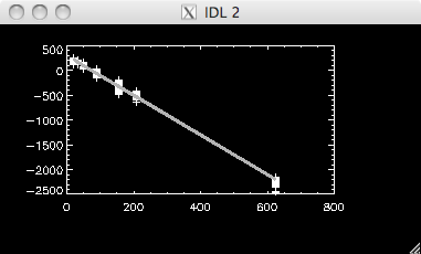

The correction factors where DC' = -3.988 & M = 302.250.

8th June 2010 I wrote a program to correct the data using the algorithm: data = incorrect_data - DC'/ Texp and to save the results. I also saved the 1-, 2- , and 3- sigma data sets (i.e. 1 standard deviation, 2 standard deviation etc....). I seem to keep making the same mistake when I am writing programs in IDL where I forget to include each dimension when assigning variables (have to remember to use (*,*,...).) The median plot looked much better than last week, but still was not as flat as I would like, and had some 'dips' on the left hand side which I should get rid of:

Corrected Data Median Values: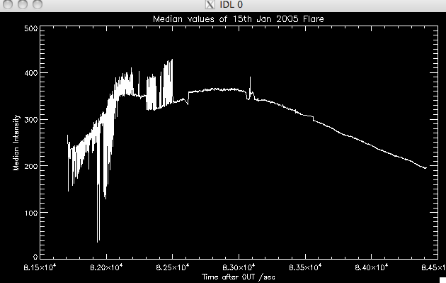

I tried selecting only a region of the quiescent sun to measure the medians, as the flaring material could be scattering photons all over the region, influencing the median values. Using the movie I made last week I identified a region which should be fairly free of flaring material and ran my find_medians program. At first there wasn't really a change, and so I started to choose smaller and smaller regions, but each time there was only a small change. 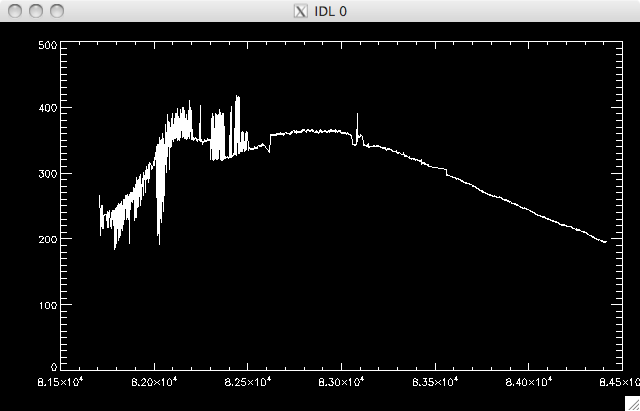Eventually I had to stop, as I couldn't be too selective of the region. So, the lack of improvement is good and bad....its bad because I want a flat-ish median plot, but good in that the median values are dominated by the quiescent sun and not the flaring sun....Jiong says that we can just normalise over the curve later. She would still like to remove the dips, and so I looked at the 3 data sets I mentioned above, which produced the following median plots:

1 sigma data set medians: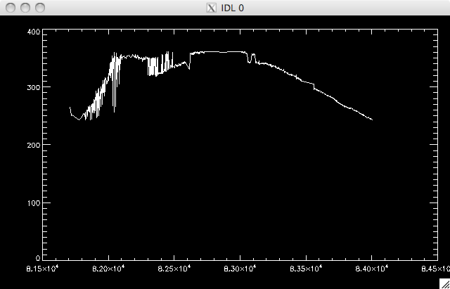

2 sigma data set medians:

3 sigma data set medians:

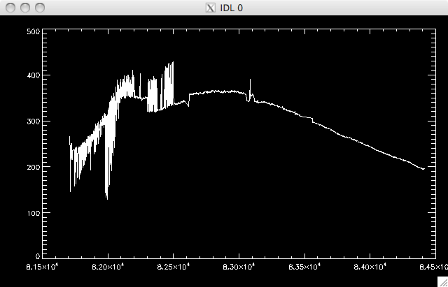As you can see, the 1-sigma data set is actually flatter and has less 'dips' but only contains ~67% of the data cube, which is not really enough to justify throwing away the rest of the data.

9th June 2010 In order to fix up the median plots, I looked at a plot of exposure time vs medians, it clear that the lowest exposure times were causing the problems:

Medians vs Exposure Times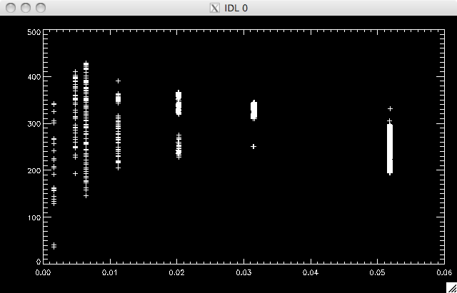

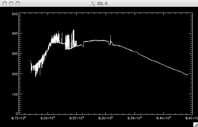
If I therefore took a sub-selection of the 2 sigma data set, omitting the values below an exposure time of 0.003seconds then I could retain over 95% of the data, and improve the data set:

Sub Selection of the 2-sigma data:

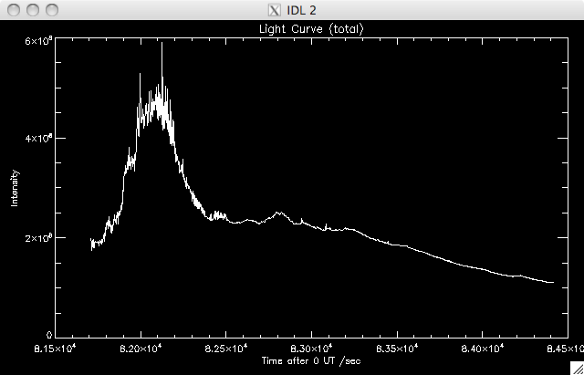
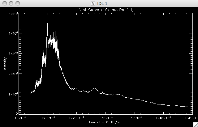
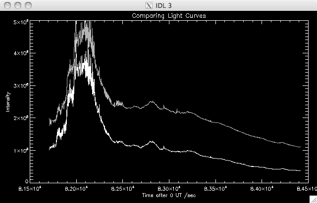
I wrote a program which took this new data and plotted light curves (the total intensity of emission at the ith time, over the duration of the flare), in a similar way to last week's program, which simply integrated up over each time frame. One plotted the total light curve for the active region, while one whittled out only the flaring material, by selecting only 10 times the median values:

Total Light Curve:

Flaring Material Light Curve:

Comparing Light Curves:

10th June 2010 Now that I have the corrected data set, and the light curves of the region, I can go onto working out the reconnection rate. I will be using a similar premise as last week, by first measuring the magnetic field, then the flux before the reconnection rate itself, but now the method will be more advanced. I adapted a set of programs Jiong gave me to do this. First I used the tessellation program to split up the SOHO magnetogram into different cells. The program found the local maximum flux (based on a scale I specified....I settled on a scale of 12 as 4 & 8 produced far more cells than I needed, and picked up loads of small changes in the background magnetic field), and then found the minimums surrounding it and drew boundaries based on this information. The different cells allows a second program to trace the evolution of magnetic evolution over the duration of the flare (the tessellation map is effectively a mask denoting the position of the cells). The data was rescaled and smoothed before finding the max and min values (the scale was set to 12 as 4 produced too many cells and picked up lots of small background differences which I was not concerned with):

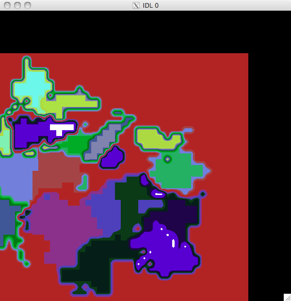
Tessellation Map (negative label = -ve flux):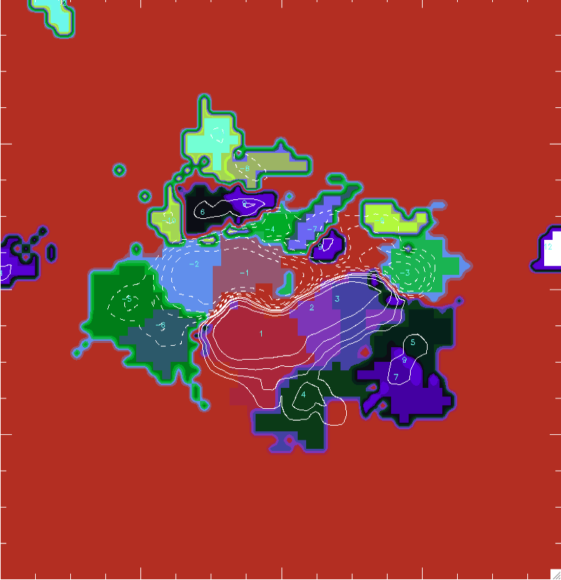

In order to overlay the tessellation map and magnetogram with the TRACE data, they had to be co aligned. The TRACE data allows me to see which pixels are brightened (more about this later). I had a high resolution MDI magnetogram [799x805] of the active region, a [512, 512] UV TRACE image, and the [799x805] tessellation map above to co align. I also had a lower resolution magnetogram [129 x 130] which was already co aligned with the TRACE image, and so I used that to help me. After some (apparently simple) geometry (and screeds of diagrams I had the images co-aligned, and could go on to find the reconnection rate. ......the co aligning involved taking the centres of the two images (SOHO & mini SOHO/TRACE) and then working out the difference between them. C' is the centre of the small map, and C is the centre of the large map: BLx = bottom left x coord, BLy = bottom left y coord, TLx = Top left x coord,.....(i'm sure you can crack the code) BLx = [lx' - lx]/ 0.5" BLy = [ly' - ly]/0.5"  where lx(') is the distance between the xcoord of the centre, C(') Lx(') = C(') - L/2 and L is the length of the edge of the image in question. I got the coordinates, in terms of pixels in the large magnetogram, which match up with the TRACE image to be: BL = (236, 164) TL = (236, 675) TR = (747, 675) BR = (747, 164) There will be errors associated here due to rounding, and due to the accuracy of the stated positions of the centres etc... but I'll deal with those next week probably.

Co aligned Tessellation map

11th June 2010 We had the Group meeting today, so I spent some time getting ready for the mini-presentation of what I've been up to. I also got started on the reconnection rate part of the analysis. Armed with my now co aligned tessellation map and magnetogram I set up my version of Jiong's program to run through a few hundred frames (just to check its working). The first part of the program will work out the flux and area of each cell and then a second program I wrote will find the reconnection rate (probably get done early next week) and the associated errors. I set up a couple of parameters to vary between different experimental runs so that I can get an estimate of the error in the measurements of flux: Cut = [6, 7, 8, 9, 10] This sets the background levels, which was cut*initial_background (set to 20 Gauss). The lower the cut, the more data which allowed past the threshold. Int = [10, 20, 30] The integration time is an effort to remove cosmic rays from the data. If you look at on the movies I posted then you'll see a bunch of flashes as point sources. These are cosmic rays, which are very fast particles registering on the ccd when they are in the line of sight. We are interested in the particles which make it down to the Sun's 'surface' and heat the material there, so it's good to remove these extraneous sources.  The int works by specifying that a pixel must remain bright for a number of frames before being considered brightened due to reconnection, i.e. for time frame i, the pixel remains bright for  i, (i + 1), (i + 2), .....(i + int-1). ..... An integration of 10 seems to be more than adequate as there are hardly any cosmic rays left. I tried int = 1, & int = 5 but these both produced a significant number of cosmic rays, so I think I'll stick with 10 from now on. An example of the plot of fluxes I have been getting is:

Magnetic Fluxes for the 5 cuts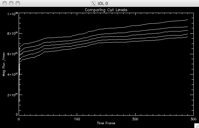

These are in the range you would expect so the program looks good to move onto the next steps. I'll vary more next time - probably the alignment of the images to get an error contribution from the co aligning process.