Week
1 Week 2
Week 3 Week 4 Week 5
Week 6 Week 7 Week 8 Week 9 Week 10
Home
Research Home
Week 6 Week 7 Week 8 Week 9 Week 10
Home
Research Home
| 12th
July 2010 Today I spent a great deal of time confirming the coalignment of TRACE and MDI. Using my previous determination as a starting point I used some routines which allowed me to manually click on an element in one image, and to click on the same element in a second image. This meant that I looked at the TRACE image for plages which had a corresponding magnetic structure. Matching up the points in each image was tricky and so I tended to err on the side of caution for most of them. Once I had selected a reasonable number of matching pairs I had IDL calculate the offset of each point, and the mean offset for the image (x & y offset) as well as the standard error. I repeated this for ~ 20 images and using the standard error for each image as a weighting factor I calculated a weighted mean and error on this mean. This gave me an offset of ~2pix by -2pix (x b y). However the standard deviation on each was ~3pix and when I performed the Flick procedure as a check, it was clear that my original estimate was better. So, although I spent a day with no real improvements I did manage to show that we had the best estimates for the image alignments and that I fall comfortably within the error we took account of (2 pixels shift when I was calculating flux). I now also have the improved PIL and so can run the position programs again. I tried this but there still seems to be an issue somewhere as the Lmax and Lmins don't make sense. Jiong thinks it is a PIL reference issue still and is going to look into solving this while I push on with the UV brightening part of the project. There is still the HXR & UV reference point difference which means we cannot yet properly compare UV & HXR positions (we can still look at trends though) so Jiong will talk to Dr Cheng to get the HXR reference and sort this. Below is a very quick example of the areas I was trying to match up. On the left is the TRACE image and on the right is the MDI image. This is a rough version I did just now to illustrate the process which is why the contour plot isn't the best. 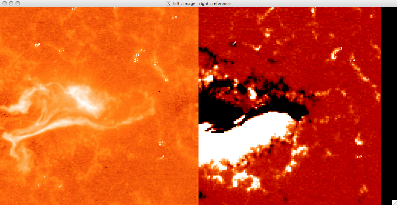 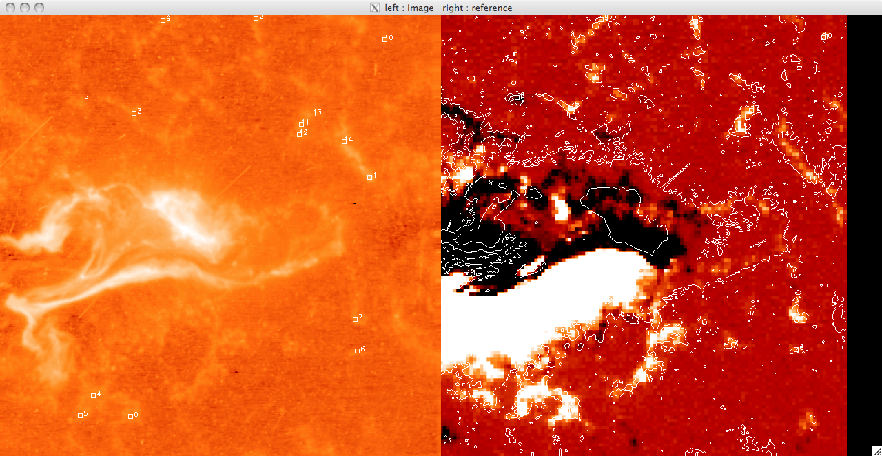 |
|
13th July 2010 Today I worked on finishing the program to select the pixels which are brightened by magnetic reconnection. I want to eventually plot the light curves with an exponential (see last week for a description of the theory behind this) and look at the decay timescales. This means that I should also identify the point at which the maximum values occur. I set an estimate of the background level based on the median values I found in the initial weeks as being 300, but this can be varied easily. Once the UV data is loaded I find the maximum across the time dimension, so that I find the maximum value that each pixel obtains over the lifetime of the flare. Once this is done I find where the maximum is greater than 50*blevel, and record these indices. I only want pixels which are brightened by reconnection, and which can be fit by a curve (i.e. they have a good light curve rather than a few spikes) so I included another layer of filtering to remove cosmic rays etc...This layer was a simple loop which stipulated that, starting from the maximum position each of the following 10 pixels must be greater than 30*blevel. This meant that they were still significantly above the background levels (i.e. still being heated) ~ 20 seconds later and unlikely to be cosmic rays. I got a surprisingly large amount of pixels (~65000 to 130000 depending on blevel and what I multiply it by) which is much more than Jiong found for the Bastille Day Flare. I'll look further into this once I see how many of these pixels can be fitted by a curve. |
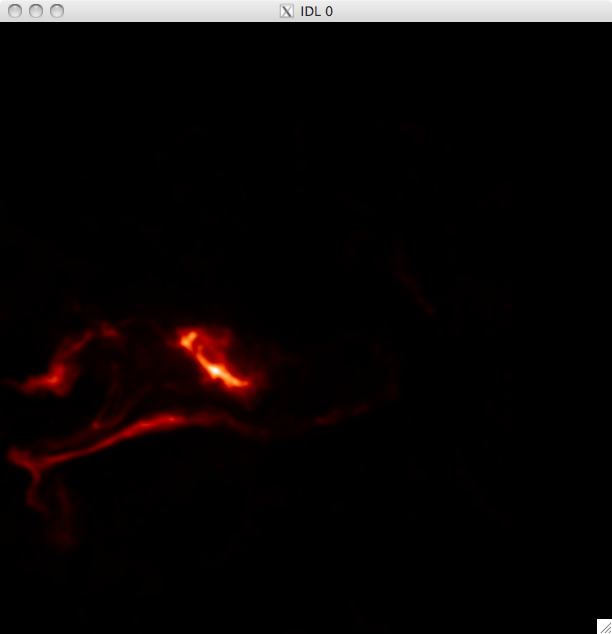
14th July 2010 Today I have been working on a program to have a quick look at the UV light curves and it seems to work out pretty well. At first I wrote it all in a test program, but I have it ready to put into my main UV pixels program. Basically, I load in the file UV data and sum up across the time dimension, which leaves me with an image highlighting the areas of flare emission (as when I total it up any regions which are brightened by hot pixels are much less intense than areas which are continually being energised and so the sum reflects this. By doing this I get a good idea of where to look for a good light curve (i.e. one due to brightening by magnetic reconnection as opposed to noise). I then use some function in IDL to allow some user input, so I can either click on a pixel, or move the cursor over it to select the x and y coordinates. I take these coords and select the pixel out of the UV data cube and plot the light curve in a separate window. I ran into some trouble where I couldn't get out of the routine without cntrl-c and so I opted to just click outside a certain range (usually the top right corner) to exit. Also, the window would showing the light curve would also disappear as soon as it appeared when the loop re-started and so it took me some time to fix this, but I just had to specify an initial click, or movement, is necessary. I also only want to see the curve if my first procedure in my UV programs identified it as being brightened, and so I converted the x & y coords into a 1D format and compared it to the array containing the indices of brightened pixels. In this way, I'm only looking at the pixels I plan to try and fit a curve to. Lastly, I included an option to show the light curves on a logarithmic scale to see if a power law would describe the data (indicating an exponential relationship) The results were encouraging- most seem exponential and also to have a possible second region which is what we were looking for. Below are several images of the light curves, and also one of the image I 'click' on to find them: |
UV Brightened Pixels:
 |
|
Light Curves: 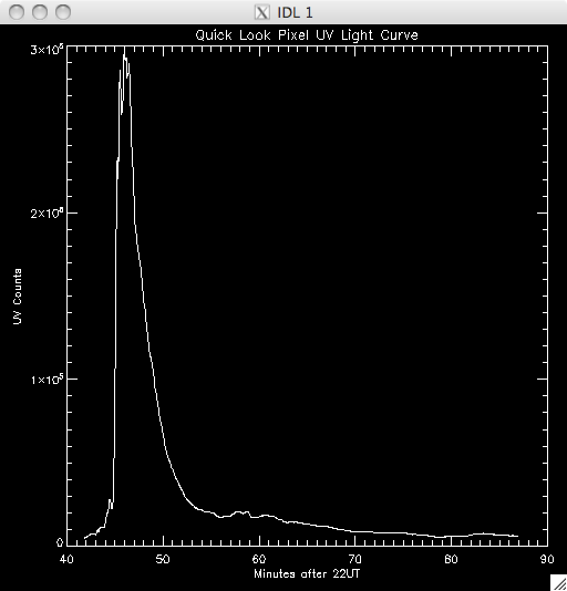 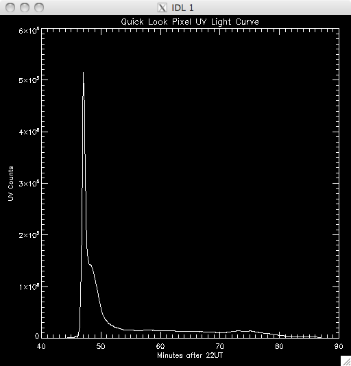 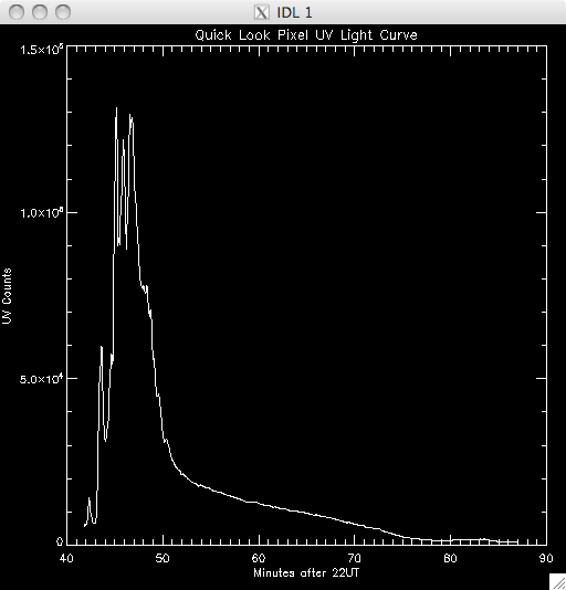 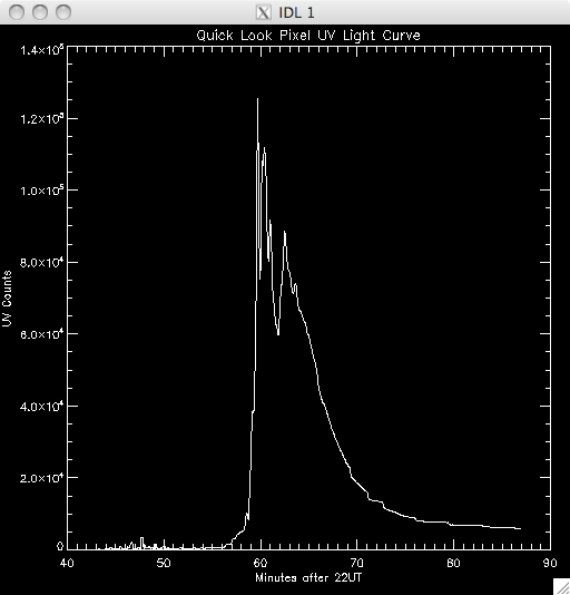 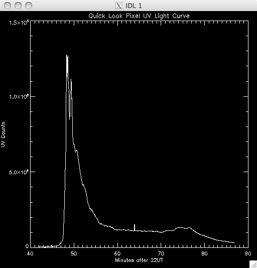 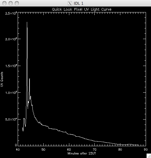 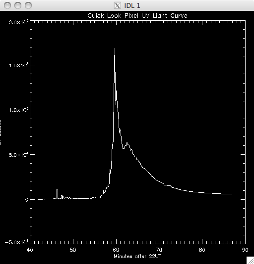 Log Scale Plots: 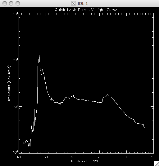 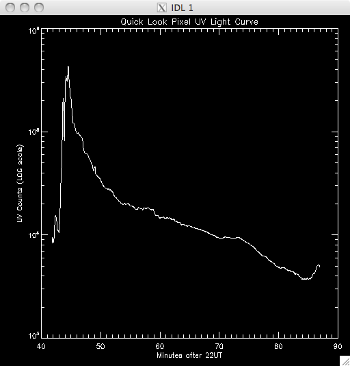 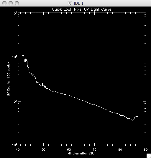 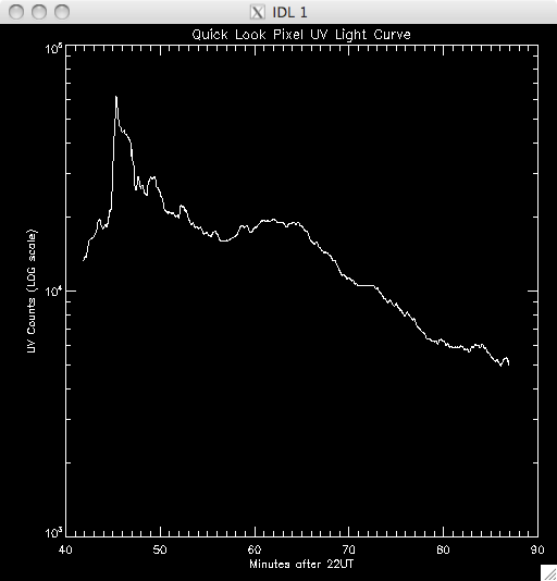 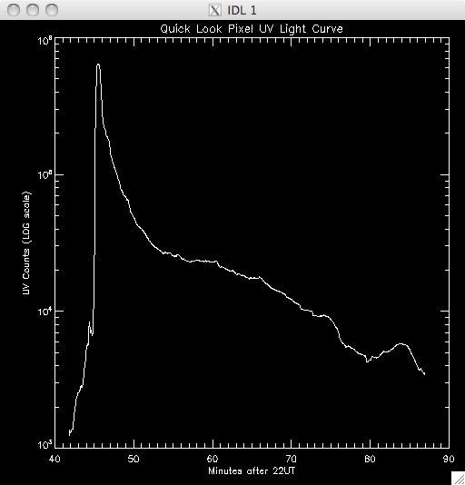 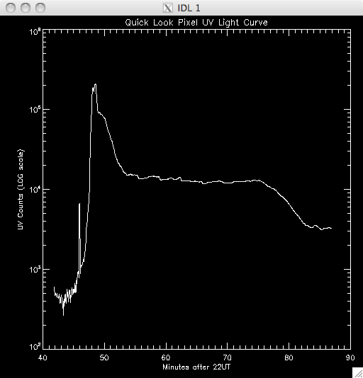 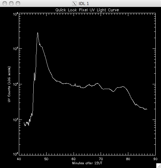 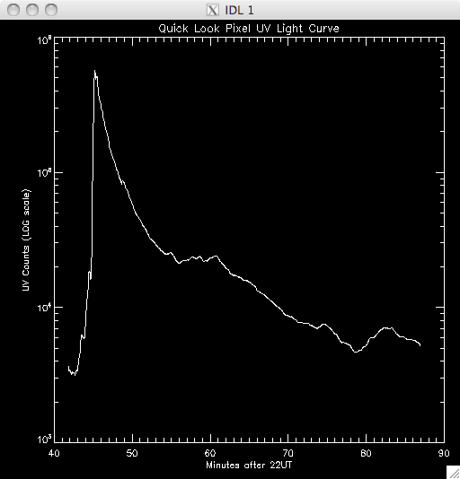 |
15th July 2010 Today a few of us went on the BOREALIS balloon launch in Harlowton which took longer than expected so I didn't get any research done, though I did have a few ideas about the fitting process I plan to write tomorrow so I should get the bulk of that done. |
16th July 2010 Today I worked on getting the program to roughly plot the UV timescales to work. Just now it only tries to fit a single power law although we suspect that there will be two power laws which model the decay of the UV- this means that most of the data will not be well-fitted by the exponential curves and so when I select the data with lower errors (i.e. close match between the fitted model and the observed data) there will not be a significant portion of the data present. However, for the moment, I want to get this program working, and I can worry about splitting the power laws up later. I also ran through the various permutations of my procedure to plot the light curves which all seemed to work and I now have them with keywords to specify whether I want to click, move the cursor or to have a log scale. From quickly looking at the light curves, and from Jiong's analysis of the Bastille Day flare we are pretty sure that an exponential should fit the data, and also that a second power law should describe the data after a certain point. To fit the first region I wrote a new procedure within my draft program, which takes the pixels which were identified as brightened and then attempts to fit an exponential curve to them. First the maximum position is found, which is taken be the Initial time T1, which has initial intensity I1, and then the last point of the region is defined. This is a little bit fuzzy as there is no generic way to define the end of the region satisfactorily and so I defined it to be some percentage of the maximum, with this maximum defined by a cut (so, 40%, 30% etc....), with the higher the cut, the less data included. So, having too low a cut means that there will be frames which could actually be from the second region seeping in, whereas too high a cut means that I am reducing the number of points to fit to (introduces more error). I set the default cut to 10% but will probably increase this after looking at the results. So the model I am trying to fit is something like : I(t) = I1 exp {-(t-T1)/tau1} where tau1 is the decay constant of the region. I linearised the expression by taking logs, and took the error to be the Poisson error on each data point. This is simply the square root of the data- and this error is inversed when taking logs. I then said that the fitting error (the error between the observed data and the model) must be less than 30% in order to count as a reasonable fit. If the data satisfied this condition then the model parameters were converted back into the form described above and were saved as a structure. I smoothed the data before doing the fit but I think it may be a better idea to smooth before finding the brightened pixels but I'll have a look at the results and decide. Obviously this program is not going to get 100% accurate fits and so the values for tau, and I1 are going to change from pixel to pixel. Hopefully they will all be around a similar value (Jiong plotted a histogram of her values for the Bastille Day flare so I'll do the same with mine). I spent most of the day writing this program and compiling my three procedures into one program so I haven't ran any data yet but I will at the start of next week. |